Mobiles Price Classification

Machine Learning

Classification

Published

April 21, 2023

Overview

This notebook investigates the use of machine learning models to classify a mobile phone price range using the following dataset.

Download Labeled Dataset (.csv)

Download Unlabeled Dataset (.csv)

The analysis covers these main steps:

Data preprocessing and Exploratory Data Analysis (EDA)
Statistical analysis for feature selection
Model training
Model evaluation

To achieve optimal model performance and understand feature dynamics, the experimental framework is implemented in the model training and evaluation which evaluates two distinct feature representation scenarios across four machine learning algorithms:

Experimental Scenarios:
- Full Feature Set.
- Statistically Selected Feature Set.
Machine Learning Algorithms:
- K-Nearest Neighbors (KNN): A distance-based classifier.
- Decision Tree: A single-tree model evaluating rule-based splits.
- Random Forest: An ensemble bagging technique combining multiple decision trees to reduce variance and capture non-linear relationships.
- XGBoost: A gradient boosting algorithm that sequentially corrects residual errors.

Additionally, hyperparameter tuning via GridSearchCV is systematically applied across all model configurations to determine optimal model parameters and prevent overfitting.

The primary objective is to perform an end-to-end machine learning process, feature selection, and model choice affect classification performance.

Install and Import Packages

%pip install --upgrade -q matplotlib joblib pandas scikit-learn scipy seaborn xgboost

import matplotlib.pyplot as plt
import pandas as pd
import seaborn as sns

Load Dataset

df = pd.read_csv('data/mobiles.csv')
df

	battery_power	blue	clock_speed	dual_sim	fc	four_g	int_memory	m_dep	mobile_wt	n_cores	...	px_height	px_width	ram	sc_h	sc_w	talk_time	three_g	touch_screen	wifi	price_range
0	842	0	2.2	0	1	0	7	0.6	188	2	...	20	756	2549	9	7	19	0	0	1	1
1	1021	1	0.5	1	0	1	53	0.7	136	3	...	905	1988	2631	17	3	7	1	1	0	2
2	563	1	0.5	1	2	1	41	0.9	145	5	...	1263	1716	2603	11	2	9	1	1	0	2
3	615	1	2.5	0	0	0	10	0.8	131	6	...	1216	1786	2769	16	8	11	1	0	0	2
4	1821	1	1.2	0	13	1	44	0.6	141	2	...	1208	1212	1411	8	2	15	1	1	0	1
...	...	...	...	...	...	...	...	...	...	...	...	...	...	...	...	...	...	...	...	...	...
1995	794	1	0.5	1	0	1	2	0.8	106	6	...	1222	1890	668	13	4	19	1	1	0	0
1996	1965	1	2.6	1	0	0	39	0.2	187	4	...	915	1965	2032	11	10	16	1	1	1	2
1997	1911	0	0.9	1	1	1	36	0.7	108	8	...	868	1632	3057	9	1	5	1	1	0	3
1998	1512	0	0.9	0	4	1	46	0.1	145	5	...	336	670	869	18	10	19	1	1	1	0
1999	510	1	2.0	1	5	1	45	0.9	168	6	...	483	754	3919	19	4	2	1	1	1	3

2000 rows × 21 columns

Data Preprocessing and EDA

First, let’s take a look at the datasets overview.

df.info()

<class 'pandas.DataFrame'>
RangeIndex: 2000 entries, 0 to 1999
Data columns (total 21 columns):
 #   Column         Non-Null Count  Dtype  
---  ------         --------------  -----  
 0   battery_power  2000 non-null   int64  
 1   blue           2000 non-null   int64  
 2   clock_speed    2000 non-null   float64
 3   dual_sim       2000 non-null   int64  
 4   fc             2000 non-null   int64  
 5   four_g         2000 non-null   int64  
 6   int_memory     2000 non-null   int64  
 7   m_dep          2000 non-null   float64
 8   mobile_wt      2000 non-null   int64  
 9   n_cores        2000 non-null   int64  
 10  pc             2000 non-null   int64  
 11  px_height      2000 non-null   int64  
 12  px_width       2000 non-null   int64  
 13  ram            2000 non-null   int64  
 14  sc_h           2000 non-null   int64  
 15  sc_w           2000 non-null   int64  
 16  talk_time      2000 non-null   int64  
 17  three_g        2000 non-null   int64  
 18  touch_screen   2000 non-null   int64  
 19  wifi           2000 non-null   int64  
 20  price_range    2000 non-null   int64  
dtypes: float64(2), int64(19)
memory usage: 328.3 KB

Based on the output above, here are some informations about the dataset. - The dataset has 2000 rows and 21 columns. - The target variable is ‘price_range’. - Notice that there is no feature with missing values. - All features are already in numerical form so that they don’t need an encoding for the categorical features.

df['price_range'].value_counts()

price_range
1    500
2    500
3    500
0    500
Name: count, dtype: int64

df['price_range'].value_counts().plot(kind='bar')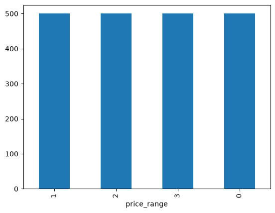

We can see that the dataset is balanced since it has exactly same number of data points for each class in the target variable ‘price_range’.

Checking dan Dropping Duplicated Rows

Let’s check the duplicated rows in train dataset and drop them if exist.

# check and drop duplicated rows (if exist)
total_duplicates = df.duplicated().sum()
print(f'Total duplicated rows: {total_duplicates}')
if total_duplicates:
    df = df.drop_duplicates()
    print('All duplicated rows has been removed.')
else:
    print('No duplicated rows need to be dropped.')

Total duplicated rows: 0
No duplicated rows need to be dropped.

Data Visualization and Feature Selection

print('-----Unique Values and Mode in Each Column-----\n\n')
all_columns = df.drop(columns=['price_range']).columns.tolist()
for column in all_columns:
    print(f'Unique Values in {column}:')
    print(df[column].unique().tolist())
    print()
    print(f'Mode: {df[column].mode()[0]}')
    print('='*50)

-----Unique Values and Mode in Each Column-----


Unique Values in battery_power:
[842, 1021, 563, 615, 1821, 1859, 1954, 1445, 509, 769, 1520, 1815, 803, 1866, 775, 838, 595, 1131, 682, 772, 1709, 1949, 1602, 503, 961, 519, 956, 1453, 851, 1579, 1568, 1319, 1310, 644, 725, 589, 1725, 790, 560, 1347, 1646, 1253, 1656, 1195, 1514, 1723, 1054, 578, 596, 1547, 1760, 1654, 1457, 1073, 1936, 823, 987, 1757, 1063, 1484, 799, 1156, 1720, 702, 616, 1358, 1242, 1166, 1448, 1407, 605, 1038, 797, 819, 1114, 1234, 1199, 1103, 1589, 999, 1510, 1008, 1127, 1412, 1496, 1083, 668, 1309, 1724, 1977, 885, 879, 1322, 1137, 1355, 1665, 657, 593, 1883, 1732, 543, 1939, 553, 832, 1661, 1657, 1135, 1775, 783, 617, 867, 1804, 1900, 909, 1084, 1308, 1778, 1701, 825, 1379, 1659, 826, 1564, 1957, 1571, 1414, 1790, 645, 1652, 1213, 1272, 866, 536, 523, 1753, 1218, 1537, 786, 1678, 1814, 1101, 1461, 1216, 506, 843, 742, 1692, 1485, 637, 1224, 1356, 1840, 1481, 1296, 1193, 1441, 517, 748, 1126, 1572, 1569, 1270, 1854, 625, 1577, 534, 946, 685, 947, 801, 703, 1165, 1082, 959, 1502, 1380, 1266, 1934, 1905, 1831, 1562, 1490, 1523, 640, 1526, 1989, 609, 1703, 1087, 671, 1472, 765, 1642, 1265, 664, 1277, 1395, 1539, 1049, 1827, 903, 1987, 1154, 1336, 1886, 1551, 850, 660, 1225, 1452, 1686, 1634, 1708, 1151, 1578, 1689, 1488, 1313, 1715, 1442, 528, 1133, 1718, 1330, 1799, 633, 724, 822, 1918, 1891, 1373, 862, 1273, 957, 1617, 893, 1210, 708, 835, 1450, 973, 601, 507, 564, 1559, 754, 728, 1431, 767, 1722, 1992, 1876, 1283, 1281, 1066, 730, 1053, 1611, 793, 1220, 1662, 538, 1733, 1429, 1839, 659, 1953, 1172, 612, 1563, 1191, 1893, 1995, 1517, 1162, 1595, 1329, 928, 1937, 977, 768, 1464, 1177, 1348, 1956, 1751, 1530, 1997, 1707, 894, 1163, 1648, 1170, 508, 1097, 1980, 1504, 1698, 920, 1144, 1430, 972, 662, 1867, 1730, 1882, 580, 1391, 1560, 821, 811, 1034, 618, 654, 576, 667, 869, 635, 1557, 1604, 1182, 848, 1610, 1828, 880, 1394, 1960, 809, 899, 1976, 916, 763, 1864, 1108, 1011, 1067, 1334, 1899, 930, 1058, 1187, 1874, 1482, 1809, 864, 1880, 1138, 1117, 1712, 1836, 1036, 1860, 1375, 1945, 1896, 788, 1323, 1868, 1042, 1479, 1476, 1552, 1454, 1007, 652, 1726, 1029, 1582, 1478, 1178, 707, 755, 912, 651, 1483, 914, 1456, 1503, 1681, 715, 1190, 1755, 1197, 1048, 1887, 1772, 1421, 954, 853, 1469, 902, 1631, 1608, 1991, 1349, 1844, 712, 1406, 1289, 932, 1747, 1128, 513, 1742, 1512, 1986, 965, 1583, 1653, 1433, 1845, 752, 1948, 1077, 1968, 1122, 1588, 1615, 1417, 1697, 1089, 1663, 1889, 857, 1902, 1554, 1337, 1926, 1278, 1773, 1438, 1846, 1260, 512, 581, 1872, 687, 1062, 1074, 1832, 1039, 1059, 1606, 1928, 1875, 1748, 1413, 535, 1780, 1671, 1076, 532, 777, 1217, 1185, 577, 737, 704, 525, 504, 569, 1590, 1350, 641, 1002, 1408, 726, 1544, 1230, 1519, 723, 1168, 1229, 1758, 1290, 574, 1271, 1269, 1288, 1366, 1627, 1974, 587, 934, 1853, 1164, 1232, 1813, 739, 1966, 1219, 1658, 1263, 621, 1175, 561, 1835, 1719, 1770, 1312, 1878, 1871, 922, 1975, 1212, 1958, 557, 539, 1369, 1109, 598, 1944, 1919, 501, 1620, 1227, 1359, 1914, 1645, 1231, 1397, 701, 570, 1993, 955, 924, 600, 518, 1841, 1762, 1112, 709, 1315, 1462, 571, 666, 1994, 966, 568, 1897, 1695, 1623, 1721, 890, 1677, 638, 852, 1979, 710, 1027, 1793, 675, 658, 1694, 804, 1713, 706, 1362, 1527, 1314, 705, 1403, 1486, 781, 986, 1567, 1940, 1717, 1254, 1591, 1640, 663, 1744, 1624, 1188, 817, 863, 1068, 1702, 808, 696, 1981, 614, 1807, 984, 720, 1536, 771, 1303, 1004, 1972, 1822, 1159, 1782, 1884, 798, 802, 1276, 1331, 1996, 1092, 1018, 545, 554, 1264, 1030, 1432, 558, 829, 1741, 1849, 733, 1149, 891, 1911, 550, 969, 1160, 827, 1786, 774, 1368, 1592, 1892, 915, 1848, 1501, 1614, 911, 1647, 967, 1204, 1320, 1800, 1439, 1422, 1929, 1511, 1852, 691, 807, 1113, 721, 805, 918, 1236, 1387, 839, 1593, 1788, 1628, 1965, 833, 1808, 1161, 787, 854, 1184, 1973, 510, 1907, 1489, 1843, 1286, 840, 757, 814, 994, 1550, 623, 1829, 1065, 1425, 642, 1664, 1498, 981, 1673, 603, 1332, 1064, 1444, 906, 841, 878, 1132, 1181, 1497, 1549, 1372, 1005, 989, 1983, 868, 1205, 1284, 626, 1763, 694, 816, 904, 979, 1531, 874, 1558, 582, 764, 743, 1061, 1428, 674, 1625, 907, 1584, 1382, 1745, 1754, 1596, 1660, 1861, 648, 1910, 1923, 1345, 1239, 516, 672, 892, 1130, 1597, 1046, 1035, 1261, 1688, 559, 860, 1090, 686, 818, 1777, 594, 1524, 511, 1402, 919, 1963, 1881, 683, 1633, 1371, 551, 1221, 1000, 1119, 1699, 1099, 1576, 950, 1081, 606, 502, 1632, 1696, 688, 1104, 1727, 1674, 531, 1057, 673, 718, 547, 812, 980, 643, 1925, 1522, 1959, 1043, 1095, 1540, 1342, 1189, 1449, 530, 1044, 1869, 1655, 1245, 846, 741, 1672, 514, 1396, 1542, 745, 1735, 586, 1341, 1970, 1545, 1729, 680, 1106, 831, 1528, 1447, 1344, 921, 1285, 1635, 1851, 727, 877, 1009, 1587, 865, 1930, 1268, 622, 1250, 1100, 815, 1031, 1136, 1300, 732, 1299, 1129, 1487, 1093, 1816, 627, 1895, 713, 1898, 1158, 1451, 1820, 1237, 1515, 1426, 1215, 697, 717, 1971, 1794, 1240, 1180, 1670, 1566, 1935, 913, 1317, 917, 1796, 740, 676, 1020, 896, 1824, 1174, 875, 1370, 991, 584, 1541, 1365, 1644, 871, 888, 1023, 1142, 1901, 1924, 1825, 1275, 1538, 1507, 948, 1384, 1766, 1811, 1988, 1423, 1446, 1398, 1885, 1436, 1998, 1321, 1339, 882, 796, 1012, 1318, 541, 1616, 1071, 1842, 1420, 1805, 610, 1533, 1801, 794, 1325, 1328, 1731, 1791, 856, 714, 951, 1759, 908, 820, 1333, 1352, 1600, 1823, 1581, 630, 1933, 1006, 1134, 599, 1392, 602, 1249, 1404, 1927, 1714, 1201, 1147, 776, 1045, 1638, 1150, 1806, 1834, 520, 565, 1143, 761, 1015, 1183, 881, 1186, 1575, 1343, 834, 844, 1335, 1650, 963, 1837, 1028, 970, 1070, 1908, 1776, 1410, 1280, 1110, 1211, 940, 729, 1494, 1546, 895, 1856, 1202, 1171, 964, 546, 1765, 1830, 1206, 1179, 744, 1148, 1676, 1001, 1086, 634, 1641, 962, 1862, 555, 1194, 1561, 1768, 936, 855, 1307, 1509, 1208, 1812, 770, 1416, 1003, 1967, 1146, 1630, 1125, 1470, 1826, 1521, 1603, 695, 1890, 1152, 1619, 1306, 1424, 942, 1922, 548, 1783, 1969, 1248, 1010, 990, 1982, 1607, 681, 753, 1779, 1855, 731, 926, 1938, 995, 993, 719, 1946, 579, 1072, 1492, 1251, 636, 1354, 583, 1203, 527, 873, 722, 628, 1207, 537, 1565, 1052, 837, 935, 665, 1493, 925, 958, 897, 1680, 983, 592, 689, 1685, 1792, 649, 1920, 1961, 608, 1802, 591, 1367, 1075, 684, 1361, 1259, 759, 1176, 1056, 1405, 1749, 1279, 544, 590, 1327, 1906, 1667, 1913, 1157, 1784, 1262, 1139, 1467, 858]

Mode: 618
==================================================
Unique Values in blue:
[0, 1]

Mode: 0
==================================================
Unique Values in clock_speed:
[2.2, 0.5, 2.5, 1.2, 1.7, 0.6, 2.9, 2.8, 2.1, 1.0, 0.9, 1.1, 2.6, 1.4, 1.6, 2.7, 1.3, 2.3, 2.0, 1.8, 3.0, 1.5, 1.9, 2.4, 0.8, 0.7]

Mode: 0.5
==================================================
Unique Values in dual_sim:
[0, 1]

Mode: 1
==================================================
Unique Values in fc:
[1, 0, 2, 13, 3, 4, 5, 7, 11, 12, 16, 6, 15, 8, 9, 10, 18, 17, 14, 19]

Mode: 0
==================================================
Unique Values in four_g:
[0, 1]

Mode: 1
==================================================
Unique Values in int_memory:
[7, 53, 41, 10, 44, 22, 24, 9, 33, 17, 52, 46, 13, 23, 49, 19, 39, 47, 38, 8, 57, 51, 21, 5, 60, 61, 6, 11, 50, 34, 20, 27, 42, 40, 64, 14, 63, 43, 16, 48, 12, 55, 36, 30, 45, 29, 58, 25, 3, 54, 15, 37, 31, 32, 4, 18, 2, 56, 26, 35, 59, 28, 62]

Mode: 27
==================================================
Unique Values in m_dep:
[0.6, 0.7, 0.9, 0.8, 0.1, 0.5, 1.0, 0.3, 0.4, 0.2]

Mode: 0.1
==================================================
Unique Values in mobile_wt:
[188, 136, 145, 131, 141, 164, 139, 187, 174, 93, 182, 177, 159, 198, 185, 196, 121, 101, 81, 156, 199, 114, 111, 132, 143, 96, 200, 88, 150, 107, 100, 157, 160, 119, 87, 152, 166, 110, 118, 162, 127, 109, 102, 104, 148, 180, 128, 134, 144, 168, 155, 165, 80, 138, 142, 90, 197, 172, 116, 85, 163, 178, 171, 103, 83, 140, 194, 146, 192, 106, 135, 153, 89, 82, 130, 189, 181, 99, 184, 195, 108, 133, 179, 147, 137, 190, 176, 84, 97, 124, 183, 113, 92, 95, 151, 117, 94, 173, 105, 115, 91, 112, 123, 129, 154, 191, 175, 86, 98, 125, 126, 158, 170, 161, 193, 169, 120, 149, 186, 122, 167]

Mode: 182
==================================================
Unique Values in n_cores:
[2, 3, 5, 6, 1, 8, 4, 7]

Mode: 4
==================================================
Unique Values in pc:
[2, 6, 9, 14, 7, 10, 0, 15, 1, 18, 17, 11, 16, 4, 20, 13, 3, 19, 8, 5, 12]

Mode: 10
==================================================
Unique Values in px_height:
[20, 905, 1263, 1216, 1208, 1004, 381, 512, 386, 1137, 248, 151, 607, 344, 356, 862, 984, 441, 658, 902, 1314, 974, 407, 466, 201, 291, 550, 511, 187, 1171, 1358, 413, 85, 178, 311, 1134, 429, 609, 347, 1448, 434, 1725, 685, 880, 1580, 186, 202, 27, 1025, 885, 1042, 1382, 546, 1013, 690, 667, 822, 581, 265, 127, 916, 361, 322, 753, 504, 651, 1565, 108, 459, 205, 570, 1172, 160, 4, 763, 339, 1040, 166, 1168, 990, 319, 1397, 708, 1077, 928, 516, 96, 666, 557, 1605, 1226, 769, 403, 177, 942, 1572, 476, 1233, 836, 824, 391, 320, 325, 125, 846, 1770, 293, 1633, 1198, 768, 70, 117, 1158, 1055, 635, 275, 1445, 1242, 597, 538, 59, 819, 179, 1259, 396, 713, 262, 622, 327, 522, 313, 226, 605, 692, 1386, 304, 1590, 229, 839, 507, 436, 756, 387, 1265, 1852, 875, 140, 577, 975, 510, 583, 674, 1125, 747, 1612, 116, 554, 811, 730, 660, 450, 1223, 1109, 45, 299, 506, 1045, 393, 650, 433, 1176, 218, 564, 986, 561, 65, 420, 1365, 619, 849, 611, 953, 642, 1417, 247, 710, 718, 1100, 938, 825, 286, 1273, 295, 852, 1277, 129, 701, 309, 213, 1112, 199, 55, 1230, 1052, 541, 809, 1738, 404, 759, 42, 397, 964, 233, 1022, 411, 954, 1528, 416, 638, 231, 574, 148, 1290, 632, 529, 1170, 169, 105, 793, 490, 1201, 246, 417, 1177, 78, 323, 707, 457, 936, 912, 1914, 526, 156, 865, 1552, 1097, 372, 1285, 302, 594, 303, 1858, 32, 590, 235, 630, 357, 475, 1054, 555, 1360, 142, 681, 104, 637, 410, 1830, 802, 56, 1053, 221, 1728, 63, 418, 854, 1869, 185, 170, 454, 866, 44, 1331, 741, 520, 114, 1153, 474, 39, 419, 584, 312, 19, 207, 363, 209, 159, 649, 1132, 1392, 1001, 712, 384, 119, 627, 1086, 195, 14, 745, 253, 333, 629, 1715, 513, 13, 1243, 300, 58, 1107, 134, 176, 1236, 336, 1116, 1010, 1453, 788, 1301, 463, 188, 1028, 1419, 1471, 168, 130, 481, 1411, 79, 1187, 77, 493, 1173, 634, 639, 431, 71, 111, 798, 408, 373, 1362, 743, 447, 30, 162, 346, 727, 180, 1641, 269, 250, 1186, 379, 264, 1486, 694, 579, 495, 315, 329, 548, 531, 191, 823, 841, 21, 966, 270, 781, 126, 228, 1091, 1452, 398, 449, 1184, 675, 1792, 1058, 592, 810, 533, 558, 1017, 765, 947, 754, 453, 282, 494, 281, 6, 292, 164, 631, 897, 268, 861, 331, 1064, 509, 957, 236, 980, 1789, 831, 636, 518, 725, 157, 1142, 840, 401, 395, 48, 982, 478, 1215, 683, 536, 83, 249, 803, 1596, 364, 946, 1428, 1613, 1127, 691, 1802, 751, 859, 206, 1673, 263, 97, 1213, 189, 628, 837, 1087, 251, 767, 389, 920, 1027, 271, 369, 1258, 1345, 613, 430, 1467, 120, 762, 600, 1350, 1597, 402, 52, 934, 214, 612, 1111, 163, 729, 1079, 338, 1698, 1108, 951, 1197, 473, 1294, 782, 464, 137, 492, 1250, 385, 427, 1024, 240, 886, 183, 88, 1016, 80, 569, 276, 1131, 551, 553, 1391, 981, 680, 687, 1060, 217, 1140, 832, 935, 446, 1308, 1002, 150, 1248, 437, 593, 693, 234, 1545, 1103, 91, 371, 1446, 181, 1311, 1791, 1568, 706, 871, 1074, 501, 833, 485, 182, 165, 192, 1156, 377, 709, 543, 113, 1114, 461, 1430, 471, 806, 204, 545, 112, 290, 1039, 1485, 1122, 462, 1384, 1502, 589, 82, 68, 689, 208, 1339, 722, 717, 1298, 618, 1214, 193, 22, 1464, 280, 337, 1036, 1347, 778, 482, 591, 901, 715, 172, 867, 451, 1119, 1299, 671, 1404, 856, 562, 997, 606, 445, 985, 1617, 375, 1795, 486, 757, 273, 491, 448, 1713, 438, 698, 965, 1399, 532, 8, 154, 198, 860, 109, 961, 243, 1626, 480, 123, 400, 190, 626, 1, 349, 1686, 1455, 95, 580, 297, 1047, 1150, 641, 653, 103, 517, 785, 761, 1179, 673, 472, 412, 977, 359, 224, 714, 843, 308, 519, 792, 382, 342, 118, 540, 18, 987, 535, 1092, 994, 210, 144, 1222, 1178, 75, 881, 351, 1842, 758, 1323, 1175, 647, 1102, 215, 945, 1096, 575, 352, 1920, 721, 777, 458, 256, 370, 1571, 573, 90, 138, 983, 149, 625, 521, 1530, 442, 152, 29, 87, 648, 341, 993, 43, 1262, 815, 1587, 750, 820, 171, 960, 624, 1295, 1164, 829, 1734, 76, 970, 578, 655, 1692, 358, 64, 259, 873, 858, 1405, 237, 1949, 335, 1638, 1480, 1220, 1011, 1081, 1512, 1136, 1145, 477, 547, 1194, 146, 1895, 1537, 821, 774, 284, 465, 705, 38, 51, 850, 426, 1578, 1463, 1432, 145, 847, 868, 663, 1749, 586, 409, 35, 1008, 952, 244, 716, 804, 787, 704, 991, 489, 1518, 855, 1261, 115, 1203, 818, 719, 1162, 330, 956, 444, 1003, 227, 334, 1281, 898, 46, 1191, 89, 368, 239, 654, 853, 686, 992, 614, 1105, 775, 1482, 737, 1211, 314, 527, 874, 657, 1209, 15, 813, 173, 378, 805, 1901, 1573, 360, 98, 703, 919, 879, 1287, 211, 890, 1260, 621, 328, 1307, 497, 219, 1163, 24, 468, 1272, 503, 1495, 1333, 267, 1070, 158, 184, 238, 800, 670, 81, 1043, 812, 274, 1438, 1157, 1511, 925, 1185, 1706, 1603, 1207, 423, 62, 405, 678, 1619, 864, 870, 1379, 220, 306, 1123, 796, 1021, 995, 1244, 1240, 194, 1076, 1238, 135, 5, 549, 838, 739, 3, 963, 1621, 887, 567, 496, 1245, 682, 724, 257, 17, 439, 153, 1699, 530, 755, 1406, 1826, 50, 817, 212, 366, 174, 882, 688, 1012, 294, 958, 1328, 354, 1709, 1099, 783, 122, 100, 1221, 599, 1274, 1878, 318, 1353, 86, 340, 602, 643, 1335, 1541, 1094, 272, 394, 903, 923, 362, 1135, 66, 924, 376, 1083, 659, 534, 285, 343, 289, 1703, 907, 287, 1151, 1085, 1078, 1750, 1475, 1836, 283, 539, 440, 0, 467, 1325, 1313, 552, 443, 576, 596, 10, 699, 23, 1063, 1421, 623, 1563, 203, 773, 332, 742, 1420, 1801, 1693, 31, 1098, 1765, 760, 2, 469, 1180, 155, 1032, 40, 1385, 672, 1088, 499, 571, 563, 944, 1138, 161, 500, 608, 277, 225, 1310, 930, 835, 664, 460, 1581, 9, 7, 278, 1288, 979, 913, 1252, 1128, 922, 1874, 484, 1015, 1303, 406, 124, 588, 776, 1117, 380, 603, 766, 1499, 988, 1618, 857, 73, 973, 245, 937, 1524, 1649, 254, 1790, 1304, 948, 1161, 242, 1569, 978, 1147, 910, 26, 1080, 744, 1466, 764, 53, 728, 1225, 367, 424, 84, 102, 258, 1279, 523, 296, 1364, 950, 1960, 808, 94, 1684, 1050, 1658, 67, 1257, 11, 889, 1284, 911, 927, 1041, 525, 348, 1899, 1188, 679, 1224, 223, 167, 487, 74, 931, 921, 1057, 616, 740, 542, 383, 1442, 1352, 266, 321, 1451, 1048, 470, 1217, 298, 36, 617, 786, 645, 1371, 1332, 428, 1546, 1210, 789, 390, 110, 1330, 317, 892, 388, 914, 1661, 665, 662, 661, 560, 1315, 479, 888, 652, 1652, 976, 455, 1196, 1694, 610, 1457, 241, 528, 915, 483]

Mode: 347
==================================================
Unique Values in px_width:
[756, 1988, 1716, 1786, 1212, 1654, 1018, 1149, 836, 1224, 874, 1005, 748, 1440, 563, 1864, 1850, 810, 878, 1064, 1854, 1385, 822, 788, 1245, 1434, 645, 1075, 1311, 1263, 1739, 654, 1152, 1919, 881, 1249, 815, 1307, 730, 1613, 967, 1932, 714, 1456, 1652, 1810, 1791, 774, 1433, 1832, 1383, 629, 1287, 804, 1036, 1449, 820, 713, 683, 969, 975, 547, 1353, 1570, 1618, 1858, 1781, 1225, 603, 1724, 1217, 1026, 638, 1413, 1242, 1071, 778, 1552, 1486, 1206, 1616, 1752, 1122, 1049, 1894, 741, 1118, 1203, 1402, 1924, 802, 1105, 1990, 1179, 891, 1684, 961, 1317, 984, 520, 902, 1504, 1634, 1796, 1846, 1869, 1471, 1974, 513, 1244, 1661, 973, 771, 989, 1954, 1338, 1712, 863, 1376, 786, 1965, 1732, 1398, 829, 792, 580, 1056, 1264, 1248, 669, 1686, 1539, 1042, 1926, 616, 1131, 1697, 536, 1269, 1298, 1967, 1025, 800, 1359, 1996, 1013, 590, 1925, 1989, 826, 1983, 1545, 1533, 621, 1272, 1729, 974, 1554, 1611, 1937, 1942, 845, 627, 842, 1737, 1199, 1740, 648, 1136, 1220, 879, 1065, 831, 1191, 1631, 588, 500, 1698, 1299, 898, 1381, 1464, 539, 751, 1497, 1215, 1948, 1542, 1235, 1345, 589, 1182, 1052, 1429, 873, 1478, 1460, 705, 1666, 1077, 1020, 1516, 1499, 583, 1958, 1995, 642, 1178, 1404, 1040, 1453, 1677, 517, 1560, 1226, 1200, 1647, 1308, 1615, 687, 637, 1606, 1543, 980, 1441, 1009, 1754, 860, 1108, 673, 1758, 886, 1485, 1038, 946, 1462, 1604, 1882, 1816, 765, 1980, 1559, 1928, 1529, 952, 1517, 1741, 1596, 1564, 1222, 692, 1617, 1571, 1247, 1767, 1935, 1933, 1509, 954, 662, 888, 527, 1493, 1929, 764, 1092, 1891, 1699, 1664, 763, 572, 1963, 1489, 1294, 997, 655, 1458, 1243, 519, 566, 515, 1168, 882, 776, 564, 1975, 1388, 1130, 754, 1726, 1876, 709, 557, 1914, 775, 1910, 1923, 1370, 994, 1078, 724, 1104, 1795, 1442, 1023, 1361, 652, 935, 1292, 1256, 1364, 682, 1688, 1898, 1438, 1463, 1584, 1059, 1253, 939, 986, 1029, 1280, 1565, 1331, 1922, 992, 1186, 1920, 1866, 981, 1195, 1706, 749, 1711, 681, 1510, 814, 1814, 1233, 721, 1670, 550, 699, 1138, 1903, 817, 1126, 1139, 926, 1506, 726, 1753, 794, 1161, 1350, 619, 660, 1468, 1705, 1476, 1033, 559, 1223, 956, 1797, 596, 574, 990, 1053, 858, 758, 1495, 1352, 1304, 1205, 562, 585, 1629, 1798, 545, 1657, 1341, 1058, 1744, 740, 1133, 889, 1719, 1285, 1905, 1158, 1325, 772, 1743, 1208, 1050, 1366, 899, 1884, 867, 884, 1358, 998, 862, 1785, 799, 793, 695, 728, 1940, 1259, 790, 1594, 548, 1911, 1649, 1262, 1972, 1484, 1090, 1439, 592, 1777, 870, 1106, 948, 1393, 982, 1586, 1579, 644, 1157, 750, 1472, 1337, 1663, 861, 773, 1313, 1849, 1151, 1807, 1763, 1827, 1916, 1580, 1582, 1234, 1917, 1759, 848, 1803, 915, 1354, 1143, 632, 1642, 1450, 1587, 1665, 1815, 739, 963, 1508, 1000, 544, 1627, 759, 1416, 1088, 760, 857, 1100, 676, 658, 1239, 1901, 1813, 1578, 1878, 1109, 1171, 1949, 1722, 1809, 964, 1237, 1082, 828, 1241, 1710, 1793, 1951, 1704, 1897, 809, 1306, 1771, 1536, 1987, 1022, 522, 1883, 1787, 910, 781, 1501, 1176, 684, 1838, 904, 1682, 1715, 906, 1230, 1315, 599, 1302, 727, 1096, 1173, 816, 1970, 1101, 1089, 901, 1701, 1232, 630, 1184, 1991, 510, 1511, 747, 1947, 1421, 672, 1031, 575, 1282, 1435, 1651, 516, 1703, 1048, 1873, 1465, 1477, 1748, 1159, 1630, 1293, 1162, 1747, 736, 1418, 757, 1750, 549, 818, 938, 1505, 1116, 991, 577, 1374, 1251, 1674, 1016, 1327, 501, 1621, 1532, 811, 1318, 1655, 1702, 1862, 1301, 1605, 718, 1742, 1558, 766, 1799, 1658, 1998, 1491, 650, 907, 1595, 895, 1589, 1384, 1733, 922, 1291, 1648, 723, 999, 1300, 819, 1238, 643, 1633, 735, 1339, 1445, 1424, 883, 1452, 806, 849, 1812, 947, 1895, 1123, 1409, 1675, 1930, 1518, 859, 821, 1671, 1865, 1448, 896, 605, 1330, 670, 1909, 1185, 1008, 1668, 1482, 1229, 823, 1326, 932, 1641, 1051, 1889, 1982, 893, 1163, 962, 697, 1312, 1469, 704, 671, 1583, 791, 1391, 1336, 1638, 690, 1073, 1660, 1395, 783, 1145, 1169, 1360, 1423, 1577, 1181, 1228, 1523, 1513, 812, 1081, 1406, 1001, 1500, 530, 832, 1267, 928, 1382, 1011, 1076, 688, 1403, 734, 1968, 1165, 1481, 1569, 1367, 1125, 1913, 1155, 618, 1084, 1723, 1514, 937, 1119, 1556, 1819, 1394, 1197, 1956, 614, 1334, 558, 507, 1190, 1973, 506, 1019, 674, 1420, 1377, 1538, 511, 541, 940, 1659, 983, 1219, 1735, 719, 1915, 917, 1808, 1908, 1977, 930, 1877, 1997, 1284, 661, 698, 1782, 1261, 1902, 1667, 1960, 1591, 890, 864, 1994, 1392, 1427, 1731, 875, 1348, 635, 622, 653, 570, 1356, 1553, 1985, 663, 1976, 1761, 1520, 1768, 631, 843, 1623, 1964, 1801, 1992, 571, 1746, 1055, 877, 830, 1805, 722, 646, 1309, 1079, 1087, 1626, 521, 1515, 710, 1401, 1432, 1637, 1068, 755, 1531, 656, 869, 1555, 1764, 1046, 594, 1896, 1320, 1687, 1069, 1170, 1347, 1324, 966, 846, 1389, 607, 1636, 1305, 1966, 1602, 1607, 1490, 1762, 1455, 556, 1014, 1411, 525, 1843, 797, 1043, 565, 887, 639, 1804, 1581, 912, 745, 1278, 1344, 1892, 1788, 1422, 1037, 551, 1841, 876, 620, 1012, 768, 807, 1335, 1544, 1378, 707, 1609, 1593, 1057, 1032, 1473, 1656, 1134, 1756, 711, 1899, 679, 1252, 1387, 1886, 1144, 613, 909, 798, 1676, 1147, 1738, 1362, 1461, 1062, 598, 1316, 1694, 1783, 1524, 1728, 1678, 1622, 979, 1310, 970, 1931, 1528, 1614, 1437, 1004, 1683, 784, 1066, 1400, 1766, 1662, 1773, 1274, 1454, 1210, 568, 533, 696, 640, 1496, 1769, 855, 1167, 1386, 1836, 941, 1039, 518, 865, 1156, 1227, 1893, 1273, 686, 1708, 1340, 581, 1709, 1981, 1681, 1007, 1027, 1527, 1619, 694, 1103, 1713, 1250, 850, 1132, 1957, 1492, 903, 540, 512, 1098, 1717, 1193, 1639, 1431, 1880, 925, 1363, 977, 978, 1551, 1857, 1240, 1021, 703, 675, 1945, 1802, 1010, 892, 636, 1407, 1567, 584, 1349, 1692, 1183, 866, 1645, 1790, 1373, 1775, 853, 1546, 569, 1405, 1776, 1727, 1780, 1718, 1399, 542, 1003, 647, 1575, 1196, 1950, 738, 851, 1175, 1806, 1944, 623, 1372, 1459, 1853, 844, 833, 761, 509, 1487, 1811, 700, 1646, 1288, 1028, 1550, 1483, 1952, 1503, 1375, 665, 1540, 1148, 1083, 1164, 770, 1207, 1848, 1829, 1673, 1180, 1258, 1127, 742, 1099, 1986, 1566, 503, 508, 1289, 1290, 1113, 1111, 957, 1035, 1115, 1150, 708, 712, 529, 839, 1851, 1030, 538, 732, 1415, 1643, 1211, 591, 918, 1794, 1817, 908, 1177, 1006, 1371, 1635, 1534, 1135, 528, 1430, 1839, 1760, 1343, 1831, 1414, 1904, 789, 1852, 1231, 1962, 951, 1129, 1351, 840, 678, 1608, 615, 725, 1888, 1436, 769, 1870, 1451, 1255, 872, 1275, 534, 1254, 1879, 1603, 593, 1800, 1912, 1696, 1141, 610, 1721, 1466, 1397, 582, 657, 1979, 1396, 537, 885, 651, 737, 854, 1426, 743, 1890, 1632]

Mode: 874
==================================================
Unique Values in ram:
[2549, 2631, 2603, 2769, 1411, 1067, 3220, 700, 1099, 513, 3946, 3826, 1482, 2680, 373, 568, 3554, 3752, 1835, 2337, 2819, 3283, 1433, 1037, 2583, 2782, 3763, 3286, 2373, 478, 3532, 508, 2227, 3845, 1262, 1326, 2113, 3429, 3169, 2150, 2484, 3339, 1878, 1629, 504, 1152, 3587, 2296, 1270, 3238, 2059, 2053, 3112, 1440, 2908, 2552, 905, 3963, 2056, 2910, 1457, 431, 470, 2148, 2955, 3366, 3068, 3834, 1050, 3993, 3378, 2192, 392, 3709, 590, 1814, 907, 1449, 3448, 1837, 3464, 2593, 3484, 2009, 2048, 837, 854, 3210, 2746, 2334, 2822, 1971, 1410, 349, 1418, 3616, 880, 1601, 1412, 1692, 2600, 1308, 2413, 1047, 1204, 1799, 2676, 2597, 3029, 2343, 2016, 2213, 790, 3182, 3472, 2871, 3187, 1945, 488, 1214, 2598, 3242, 3534, 3426, 2488, 3255, 2863, 1496, 3801, 666, 3799, 1366, 2962, 2399, 2338, 2700, 2235, 3825, 284, 1427, 1324, 398, 3685, 2390, 278, 3556, 2196, 2268, 2965, 2341, 3557, 1354, 2147, 505, 1394, 374, 506, 3702, 1078, 2945, 2981, 490, 536, 2317, 3704, 2126, 2050, 2462, 1260, 3770, 1886, 3323, 2060, 3926, 2177, 728, 2478, 2842, 1617, 1472, 764, 3965, 3693, 797, 1687, 2940, 1545, 2505, 2243, 3600, 3971, 2844, 1665, 3355, 1866, 1287, 1046, 1441, 690, 2504, 2677, 2984, 1362, 3629, 3559, 2571, 2107, 1022, 711, 3117, 978, 1869, 1179, 3844, 593, 588, 3836, 2669, 2958, 3031, 3388, 2377, 2458, 2766, 3054, 3791, 625, 3256, 707, 3755, 1733, 720, 3560, 2311, 3846, 1717, 3800, 1767, 1846, 829, 2986, 2394, 2169, 1181, 575, 2977, 532, 1702, 1074, 3352, 1027, 2039, 461, 527, 3271, 606, 2513, 1675, 2698, 1129, 468, 1210, 3086, 1595, 2332, 2589, 3760, 1851, 417, 294, 3576, 3945, 927, 2044, 1477, 3161, 3660, 1604, 2211, 3822, 3922, 1203, 447, 1652, 3608, 1228, 1499, 3321, 1206, 952, 3927, 311, 955, 1109, 2969, 725, 1655, 3490, 1774, 3615, 714, 2768, 3739, 610, 715, 663, 1725, 834, 3865, 3059, 651, 796, 785, 3252, 1322, 2832, 1615, 2125, 990, 1213, 2500, 2801, 3451, 1201, 3139, 1938, 3185, 2111, 2369, 3625, 1051, 1036, 2938, 2855, 2727, 2973, 2581, 2690, 916, 2563, 3359, 941, 2280, 827, 473, 1274, 364, 3699, 2927, 1470, 2616, 2915, 2686, 1243, 3264, 2261, 2993, 706, 2542, 2523, 336, 2457, 418, 3917, 1246, 2971, 2324, 3121, 3333, 3475, 2360, 2895, 3652, 3097, 2101, 3918, 3869, 732, 3684, 3969, 1414, 1892, 3131, 2532, 3215, 1529, 2403, 3419, 3648, 1974, 2806, 2239, 582, 3890, 1141, 2511, 3838, 2734, 2330, 2244, 808, 1587, 2492, 2122, 1122, 3021, 624, 3937, 1797, 1458, 3348, 1834, 2775, 1277, 457, 438, 985, 3701, 1052, 1175, 1070, 3411, 301, 489, 2756, 2612, 1724, 2190, 1900, 3915, 1043, 3817, 2362, 1107, 2982, 2042, 1343, 2610, 2335, 1614, 1138, 604, 3955, 258, 1066, 1731, 3860, 3630, 1965, 1459, 2323, 3291, 3272, 918, 3488, 3961, 463, 3644, 1713, 429, 2765, 2084, 1125, 1223, 3672, 3100, 343, 1970, 2728, 3635, 2180, 3864, 1155, 3566, 864, 869, 591, 1333, 2208, 1955, 3416, 3803, 574, 2129, 1948, 2978, 1619, 3716, 3454, 3777, 2712, 1434, 3968, 3383, 3278, 3970, 2674, 2776, 2336, 2430, 891, 3886, 1711, 2856, 2447, 814, 2951, 3653, 1891, 701, 2811, 1701, 1853, 2445, 2287, 2003, 3595, 1726, 3952, 850, 1446, 1300, 719, 988, 2606, 2912, 2339, 1028, 3173, 1667, 1897, 3269, 445, 1073, 665, 3129, 3501, 3461, 3206, 3717, 861, 2885, 2777, 1017, 980, 3309, 3607, 1257, 759, 3720, 475, 1336, 1185, 705, 3483, 1183, 3373, 565, 3153, 3421, 316, 448, 2366, 3881, 462, 1480, 1087, 2711, 2144, 1165, 2998, 2249, 752, 1409, 3072, 1305, 3597, 3132, 3856, 1524, 3673, 3293, 3035, 584, 2675, 2382, 1391, 2346, 1076, 643, 783, 3809, 2104, 1762, 3137, 1756, 3663, 2437, 1432, 1620, 961, 2608, 514, 2304, 933, 1896, 3655, 1973, 2183, 824, 1254, 3622, 1704, 1624, 2574, 950, 273, 446, 1510, 751, 3393, 3771, 2735, 2253, 452, 1419, 969, 3441, 3786, 2710, 3533, 1735, 2298, 2027, 2406, 2419, 995, 2078, 1145, 626, 1509, 3371, 297, 3508, 2385, 1301, 2167, 3914, 2312, 2297, 411, 3226, 740, 3878, 3406, 2440, 3959, 3703, 3714, 337, 3176, 1205, 2473, 1229, 2896, 520, 1378, 3254, 1803, 2501, 3762, 1796, 2630, 1380, 3487, 3015, 3204, 433, 1906, 898, 2799, 2020, 770, 305, 2953, 1671, 3772, 2870, 2577, 2246, 2405, 3377, 3619, 1184, 3713, 3798, 1026, 1086, 2236, 1303, 3048, 616, 3764, 419, 2858, 820, 3387, 3447, 1403, 2295, 2073, 3872, 302, 1519, 404, 595, 1663, 2764, 2614, 1094, 2826, 2496, 2103, 966, 2172, 3916, 3902, 2487, 363, 3233, 3076, 1513, 542, 3481, 3991, 1790, 509, 282, 3006, 1913, 3746, 3941, 3925, 424, 1284, 277, 485, 3002, 2893, 1406, 629, 3724, 3835, 2376, 3438, 2655, 3361, 3535, 2587, 2736, 676, 2941, 3336, 3796, 3654, 2934, 2889, 3315, 1993, 2509, 3165, 286, 776, 3213, 716, 3486, 3237, 1944, 1436, 3190, 1334, 3657, 2080, 1609, 3078, 1968, 3358, 1539, 942, 3669, 3612, 2351, 1285, 515, 654, 2540, 3412, 2547, 1369, 2942, 2812, 3497, 619, 1475, 1950, 3592, 3573, 1329, 3568, 1947, 1998, 3302, 3884, 1656, 911, 3892, 3897, 656, 1653, 860, 2197, 3458, 2066, 3676, 1518, 1018, 1360, 3449, 2524, 703, 1251, 1732, 1252, 2146, 1927, 3328, 1172, 3598, 1511, 3119, 3647, 3148, 2829, 3998, 999, 1808, 589, 3317, 670, 2173, 1561, 1401, 1275, 1464, 3019, 1083, 3538, 2493, 3726, 1531, 601, 2991, 3912, 309, 323, 1489, 3731, 667, 1241, 3142, 1444, 934, 3863, 3506, 348, 550, 971, 3984, 2019, 1870, 1352, 570, 546, 3624, 2944, 1209, 2752, 3868, 3087, 947, 1484, 347, 3227, 3299, 2641, 2622, 929, 1211, 511, 3034, 2438, 3744, 1377, 3520, 1699, 1095, 325, 1649, 1898, 2609, 2265, 1445, 356, 523, 3745, 1402, 2085, 587, 2030, 816, 3705, 2800, 3773, 1754, 1904, 2705, 3537, 1370, 1222, 3102, 2648, 3162, 1368, 724, 912, 2784, 793, 560, 312, 545, 1591, 893, 2514, 1032, 819, 3833, 2043, 1816, 2166, 2469, 2575, 1375, 673, 2301, 1781, 2248, 921, 391, 1719, 3262, 2693, 441, 1267, 687, 2890, 1737, 887, 2389, 3431, 3601, 2459, 3230, 3646, 2200, 3862, 3077, 621, 2372, 2857, 3143, 3197, 2262, 815, 3022, 2573, 2678, 1282, 2074, 1080, 2867, 1075, 3063, 2479, 2814, 2094, 2315, 2519, 735, 1386, 3260, 2022, 1716, 1454, 2290, 3940, 2219, 2495, 2361, 1783, 931, 1344, 1882, 2865, 757, 3469, 3300, 2719, 3012, 2836, 594, 2968, 892, 467, 345, 3033, 2110, 3105, 874, 3681, 737, 315, 2286, 2392, 1857, 3305, 959, 2635, 1936, 3637, 896, 2349, 774, 3397, 3964, 1887, 2114, 1542, 3038, 2481, 841, 3565, 1958, 2454, 3392, 262, 530, 2562, 2632, 259, 688, 2554, 3859, 571, 402, 878, 2130, 454, 2638, 1824, 876, 2706, 659, 455, 2378, 2278, 3436, 3424, 401, 681, 3212, 2036, 1642, 3465, 3900, 1105, 2064, 1142, 1060, 2381, 1339, 2560, 285, 2476, 1862, 3178, 733, 756, 1905, 2636, 2014, 3056, 465, 1108, 851, 1430, 362, 2456, 3700, 2620, 437, 3774, 1218, 696, 3407, 2086, 1356, 3571, 2132, 3209, 2096, 1273, 3623, 368, 3130, 3784, 3885, 1494, 1471, 2001, 1486, 1321, 1877, 3499, 2124, 1221, 2316, 1068, 1930, 1316, 1742, 3265, 2115, 3144, 1571, 1817, 3340, 2790, 577, 3593, 1355, 832, 436, 722, 2802, 1780, 1247, 3066, 403, 2518, 1069, 2651, 2974, 657, 3372, 1628, 3721, 763, 792, 1568, 1276, 2520, 3423, 1868, 2171, 780, 712, 1012, 318, 3948, 1161, 3707, 2926, 471, 1220, 2754, 1005, 2439, 2302, 857, 3518, 2821, 3442, 1309, 1812, 1384, 1348, 3957, 1212, 1382, 838, 378, 909, 3632, 3396, 1861, 2528, 1280, 2189, 531, 2331, 794, 2644, 1666, 2157, 1196, 2072, 1590, 2916, 726, 3577, 2627, 685, 1693, 2137, 3696, 1342, 1379, 1164, 908, 1019, 2299, 3011, 1543, 3692, 2753, 2156, 2637, 331, 3073, 422, 2293, 3958, 432, 298, 3847, 1921, 2423, 1658, 2289, 2182, 2184, 2872, 2367, 1919, 3296, 1593, 2933, 3154, 3563, 1907, 324, 1404, 2738, 2722, 2294, 1424, 1133, 555, 3785, 3675, 435, 3183, 3495, 2647, 702, 1836, 3894, 2424, 2671, 1146, 1422, 1115, 456, 2750, 2273, 2355, 2328, 558, 1345, 425, 1208, 267, 3122, 2929, 1598, 2052, 1249, 412, 263, 639, 1550, 1646, 3695, 3235, 2258, 1825, 3887, 1813, 817, 3614, 2013, 543, 3400, 2623, 1400, 3127, 2803, 3564, 2515, 3930, 3476, 2666, 1695, 3510, 2033, 1686, 862, 957, 3494, 3083, 313, 3282, 1149, 3899, 2785, 3761, 2240, 1875, 920, 361, 1540, 1077, 3610, 512, 3024, 1610, 2201, 3338, 3473, 2203, 940, 1798, 1567, 1491, 3905, 291, 1788, 3322, 1751, 1641, 2854, 3115, 3259, 1612, 2319, 1258, 3555, 524, 3541, 3437, 1637, 3064, 1393, 1633, 3284, 464, 1234, 292, 2521, 2658, 879, 1743, 3330, 562, 1659, 1338, 2992, 3249, 2725, 586, 804, 2460, 1295, 2625, 1999, 3742, 1193, 3511, 885, 1044, 2548, 3966, 2757, 1794, 3933, 3094, 256, 1365, 2049, 3241, 867, 2175, 609, 3285, 3586, 2322, 354, 2308, 1082, 3104, 2847, 2256, 1113, 3990, 984, 1622, 2967, 1167, 2715, 1734, 2259, 2921, 1244, 2090, 2131, 3362, 1053, 3124, 1672, 1552, 3202, 1302, 2359, 3314, 440, 2002, 3167, 3480, 2466, 1337, 1462, 503, 708, 2029, 308, 552, 2082, 3996, 1795, 2004, 2083, 2661, 1903, 3779, 3904, 265, 1417, 1769, 2948, 2572, 3267, 2402, 3376, 1507, 641, 1607, 3521, 881, 769, 650, 3736, 739, 686, 3943, 2633, 3911, 3297, 3141, 3351, 991, 3248, 493, 1747, 2517, 1389, 2522, 1885, 704, 953, 928, 3839, 299, 340, 3606, 799, 3756, 2787, 3208, 3585, 2282, 968, 2391, 1534, 755, 1341, 1456, 3155, 773, 1829, 3883, 1647, 3548, 2694, 2195, 2506, 3767, 1150, 2321, 3433, 872, 1503, 3430, 2470, 1396, 2668, 2452, 1871, 1112, 967, 2498, 387, 635, 2023, 2215, 3851, 495, 2358, 1744, 1832, 2313, 2216, 1850, 2592, 296, 3579, 1180, 3962, 3978, 668, 2032, 3057, 3919]

Mode: 1229
==================================================
Unique Values in sc_h:
[9, 17, 11, 16, 8, 13, 19, 5, 14, 18, 7, 10, 12, 6, 15]

Mode: 17
==================================================
Unique Values in sc_w:
[7, 3, 2, 8, 1, 10, 9, 0, 15, 13, 5, 11, 4, 12, 6, 17, 14, 16, 18]

Mode: 1
==================================================
Unique Values in talk_time:
[19, 7, 9, 11, 15, 10, 18, 5, 20, 12, 13, 2, 4, 3, 16, 6, 14, 17, 8]

Mode: 7
==================================================
Unique Values in three_g:
[0, 1]

Mode: 1
==================================================
Unique Values in touch_screen:
[0, 1]

Mode: 1
==================================================
Unique Values in wifi:
[1, 0]

Mode: 1
==================================================

Train-Test Split

Split the the data into train and test set. Here, we are using 80:20 ratio for the train and test set.

from sklearn.model_selection import train_test_split

# separate the target variable
target = 'price_range'
y = df[target].values

X_df = df.drop(columns=[target])

# split the data into train and test set
X_train_df, X_test_df, y_train, y_test = train_test_split(X_df, y, test_size=0.2, random_state=42)
print(f'X_train_df shape: {X_train_df.shape}')
print(f'X_test_df shape: {X_test_df.shape}')
print(f'y_train shape: {y_train.shape}')
print(f'y_test shape: {y_test.shape}')

X_train_df shape: (1600, 20)
X_test_df shape: (400, 20)
y_train shape: (1600,)
y_test shape: (400,)

X_train_df.head()

	battery_power	blue	clock_speed	dual_sim	fc	four_g	int_memory	m_dep	mobile_wt	n_cores	pc	px_height	px_width	ram	sc_h	sc_w	talk_time	three_g	touch_screen	wifi
968	1923	0	0.5	1	7	0	46	0.5	191	1	10	767	1759	1489	10	9	3	1	1	1
240	633	1	2.2	0	0	1	49	0.1	139	8	1	529	1009	3560	11	1	16	1	1	1
819	1236	0	0.9	1	2	1	57	0.1	188	1	14	517	809	1406	14	12	20	1	0	1
692	781	0	1.1	0	2	0	38	0.4	198	5	7	304	1674	3508	13	8	5	0	0	1
420	1456	1	0.5	1	7	0	7	0.4	105	5	12	823	1104	1587	6	5	20	1	0	1

X_test_df.head()

	battery_power	blue	clock_speed	dual_sim	fc	four_g	int_memory	m_dep	mobile_wt	n_cores	pc	px_height	px_width	ram	sc_h	sc_w	talk_time	three_g	touch_screen
1860	1646	0	2.5	0	3	1	25	0.6	200	2	5	211	1608	686	8	6	11	1	1
353	1182	0	0.5	0	7	1	8	0.5	138	8	16	275	986	2563	19	17	19	1	0
1333	1972	0	2.9	0	9	0	14	0.4	196	7	18	293	952	1316	8	1	8	1	1
905	989	1	2.0	0	4	0	17	0.2	166	3	19	256	1394	3892	18	7	19	1	1
1289	615	1	0.5	1	7	0	58	0.5	130	5	8	1021	1958	1906	14	5	5	1	0

y_train

array([1, 2, 0, ..., 2, 3, 1], shape=(1600,))

y_test

array([0, 2, 1, 3, 1, 1, 2, 0, 3, 1, 0, 0, 2, 3, 3, 2, 3, 3, 1, 0, 0, 2,
       1, 2, 0, 1, 3, 2, 2, 0, 0, 0, 3, 0, 1, 1, 2, 0, 3, 0, 2, 3, 2, 0,
       2, 3, 2, 1, 3, 1, 3, 1, 0, 0, 1, 0, 1, 3, 0, 0, 1, 3, 3, 1, 0, 0,
       3, 3, 1, 2, 2, 2, 0, 1, 2, 0, 1, 3, 2, 2, 3, 2, 1, 0, 1, 3, 1, 3,
       3, 0, 3, 3, 2, 1, 3, 2, 2, 3, 1, 1, 0, 0, 1, 0, 0, 3, 2, 0, 1, 1,
       0, 0, 3, 1, 3, 2, 3, 2, 0, 2, 1, 3, 2, 1, 3, 3, 0, 2, 0, 2, 3, 0,
       2, 2, 0, 3, 1, 0, 0, 2, 2, 1, 3, 2, 0, 0, 0, 1, 1, 2, 3, 1, 1, 0,
       2, 2, 0, 1, 0, 2, 2, 3, 3, 2, 1, 0, 1, 2, 2, 3, 3, 0, 1, 0, 3, 1,
       1, 2, 1, 0, 0, 0, 0, 0, 3, 2, 0, 3, 0, 0, 0, 0, 1, 3, 3, 1, 0, 1,
       1, 1, 1, 2, 2, 3, 3, 3, 1, 2, 0, 0, 0, 2, 1, 1, 3, 1, 0, 2, 1, 1,
       3, 2, 3, 0, 0, 2, 1, 3, 0, 1, 2, 0, 2, 3, 2, 0, 1, 3, 3, 0, 1, 3,
       2, 3, 0, 3, 1, 2, 3, 3, 2, 1, 0, 3, 3, 1, 3, 3, 3, 3, 3, 0, 1, 2,
       2, 2, 3, 0, 2, 3, 2, 2, 2, 1, 0, 2, 0, 3, 3, 1, 3, 1, 0, 3, 1, 2,
       0, 0, 3, 0, 1, 2, 3, 3, 3, 1, 1, 0, 1, 3, 3, 0, 1, 2, 2, 0, 3, 3,
       2, 3, 2, 3, 2, 0, 2, 1, 1, 1, 0, 0, 0, 3, 3, 3, 1, 0, 1, 0, 2, 2,
       3, 0, 3, 3, 2, 1, 3, 0, 0, 2, 1, 3, 2, 0, 1, 1, 1, 1, 1, 3, 2, 0,
       0, 3, 3, 0, 3, 0, 0, 2, 0, 1, 2, 2, 2, 3, 0, 3, 2, 3, 3, 3, 3, 2,
       1, 1, 0, 3, 1, 3, 3, 0, 2, 3, 2, 3, 3, 3, 0, 0, 2, 3, 0, 0, 2, 3,
       2, 1, 1, 2])

For the next exploratory data analysis, it is conducted exclusively on the Training Set. The Test Set remains completely untouched and unseen, acting as pure out-of-sample data to ensure an unbiased evaluation of the final model. Then, divide the training dataset into 2 parts: numerical features only and categorical features only.

# divide the dataframe into 2 parts: numerical features only and categorical features only
cat_columns = ['blue', 'dual_sim', 'four_g', 'three_g', 'touch_screen', 'wifi']
num_columns = list(set(X_df.columns) - set(cat_columns))

X_train_cat_df = X_train_df[cat_columns]
X_train_num_df = X_train_df[num_columns]

print(f'X_train_cat_df shape: {X_train_cat_df.shape}')
print(f'X_train_num_df shape: {X_train_num_df.shape}')

X_train_cat_df shape: (1600, 6)
X_train_num_df shape: (1600, 14)

Categorical Features

Let’s create grouped bar charts to visualize the categorical features.

countplot_df = X_train_cat_df.copy()
countplot_df[target] = y_train

n_columns = 3
n_rows = (len(num_columns) + n_columns - 1) // n_columns

fig, axes = plt.subplots(n_rows, n_columns, figsize=(15, 5 * n_rows))
axes = axes.flatten()

for i, column in enumerate(cat_columns):
    sns.countplot(data=countplot_df, x=target, hue=column, ax=axes[i])

for j in range(i + 1, len(axes)):
    fig.delaxes(axes[j])

plt.show()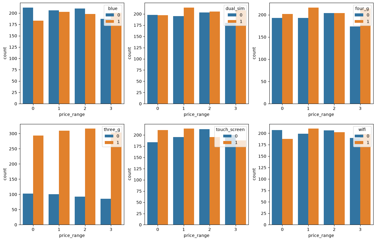

This side-by-side bar symmetry demonstrates that the presence or absence of these hardware features occurs with equal probability regardless of the smartphone’s price level. The visual lack of skewness or concentration reinforces that these binary features are statistically independent of the target, providing further empirical justification for pruning them during the Chi-Square feature selection process.

To determine which categorical features hold significant predictive power over the categorical target variable (price_range), Chi-Square Test of Independence is employed.

The Chi-Square Test of Independence evaluates whether a significant association exists between two categorical variables by comparing the Observed Frequencies (\(O\)) in the sample data against the Expected Frequencies (\(E\)).

How Expected Frequencies Measure Independence

In probability theory, if two events \(A\) and \(B\) are statistically independent (i.e., having no association), the joint probability of both events occurring simultaneously is the product of their individual probabilities:

\[P(A \cap B) = P(A) \times P(B)\]

In the context of contingency tables, the Expected Frequency (\(E_{i,j}\)) for a specific cell—representing the count we would mathematically expect if the feature and the target class were completely unrelated—is computed as:

\[E_{i,j} = \frac{\text{Row Total}_i \times \text{Column Total}_j}{\text{Grand Total (N)}}\]

Measuring Association via Deviation The Chi-Square statistic quantifies the total normalized deviation between reality (\(O\)) and the assumption of independence (\(E\)):

\[\chi^2 = \sum \frac{(O_{i,j} - E_{i,j})^2}{E_{i,j}}\]

Small \(\chi^2\) value (\(p \ge 0.05\)): The observed distribution aligns closely with the expected distribution under independence. This indicates that knowing the categorical feature provides no statistically significant information about the target variable (\(\text{price\_range}\)). Thus, the feature is identified as noise and candidate for removal.
Large \(\chi^2\) value (\(p < 0.05\)): The observed frequencies diverge significantly from the independence baseline. This confirms a statistically significant association with the target, justifying the retention of the feature for machine learning modeling.

from scipy.stats import chi2_contingency

chi2_df = X_train_cat_df.copy()
chi2_df[target] = y_train

chi2_results = []

print('----- Running Chi-Square Independence Test -----\n')

for column in cat_columns:
    contingency_table = pd.crosstab(chi2_df[column], chi2_df[target])
    
    chi2_stat, p_val, dof, expected = chi2_contingency(contingency_table)

    chi2_results.append({'Feature': column,
                         'Chi-Square Stat': chi2_stat,
                         'P-Value': p_val})
    
chi2_summary_df = pd.DataFrame(chi2_results).sort_values(by='Chi-Square Stat', ascending=False).reset_index(drop=True)
print('Results:\n')
print(chi2_summary_df)

# select features with p-value < 0.05
selected_cat = chi2_summary_df[chi2_summary_df['P-Value'] < 0.05]['Feature'].tolist()
print(f'\nSelected Categorical Features: {selected_cat}\n')
print(f'Number of Selected Categorical Features: {len(selected_cat)} Out of {len(cat_columns)} Categorical Features.')

----- Running Chi-Square Independence Test -----

Results:

        Feature  Chi-Square Stat   P-Value
0  touch_screen         3.733835  0.291677
1          blue         2.447575  0.484840
2        four_g         2.387007  0.496058
3       three_g         2.100655  0.551780
4      dual_sim         1.476924  0.687606
5          wifi         1.403940  0.704611

Selected Categorical Features: []

Number of Selected Categorical Features: 0 Out of 6 Categorical Features.

A comprehensive evaluation of the binary/categorical features (blue, dual_sim, four_g, three_g, touch_screen, and wifi) indicates that these attributes exert virtually no meaningful impact on determining a smartphone’s price range.

Visual Evidence: Across the grouped bar charts, any of the four target price ranges (\(\text{price\_range} \in \{0, 1, 2, 3\}\)) hover uniformly around 25% for both binary states (\(0\) and \(1\)). The lack of structural deviation or concentration in specific cells visually confirms that these features are distributed at random relative to the price categories.
Statistical Confirmation (Chi-Square Test of Independence): This visual independence is rigorously backed by the Chi-Square test of independence. The calculated \(\chi^2\) values for all categorical features are small, yielding \(p\text{-values} > 0.05\). Consequently, we fail to reject the null hypothesis (\(H_0\)), confirming that these binary hardware specifications share no statistically significant association with price_range. Retaining them would only introduce irrelevant noise into distance-based estimators like KNN.

Numerical Features

Let’s also explore which numerical features have a strong relationship with the target variable by creating box plots.

boxplot_df = X_train_num_df.copy()
boxplot_df[target] = y_train

n_columns = 3
n_rows = (len(num_columns) + n_columns - 1) // n_columns

fig, axes = plt.subplots(n_rows, n_columns, figsize=(15, 5 * n_rows))
axes = axes.flatten()

for i, column in enumerate(num_columns):
    sns.boxplot(boxplot_df, x=target, y=column, ax=axes[i])

for j in range(i + 1, len(axes)):
    fig.delaxes(axes[j])

plt.show()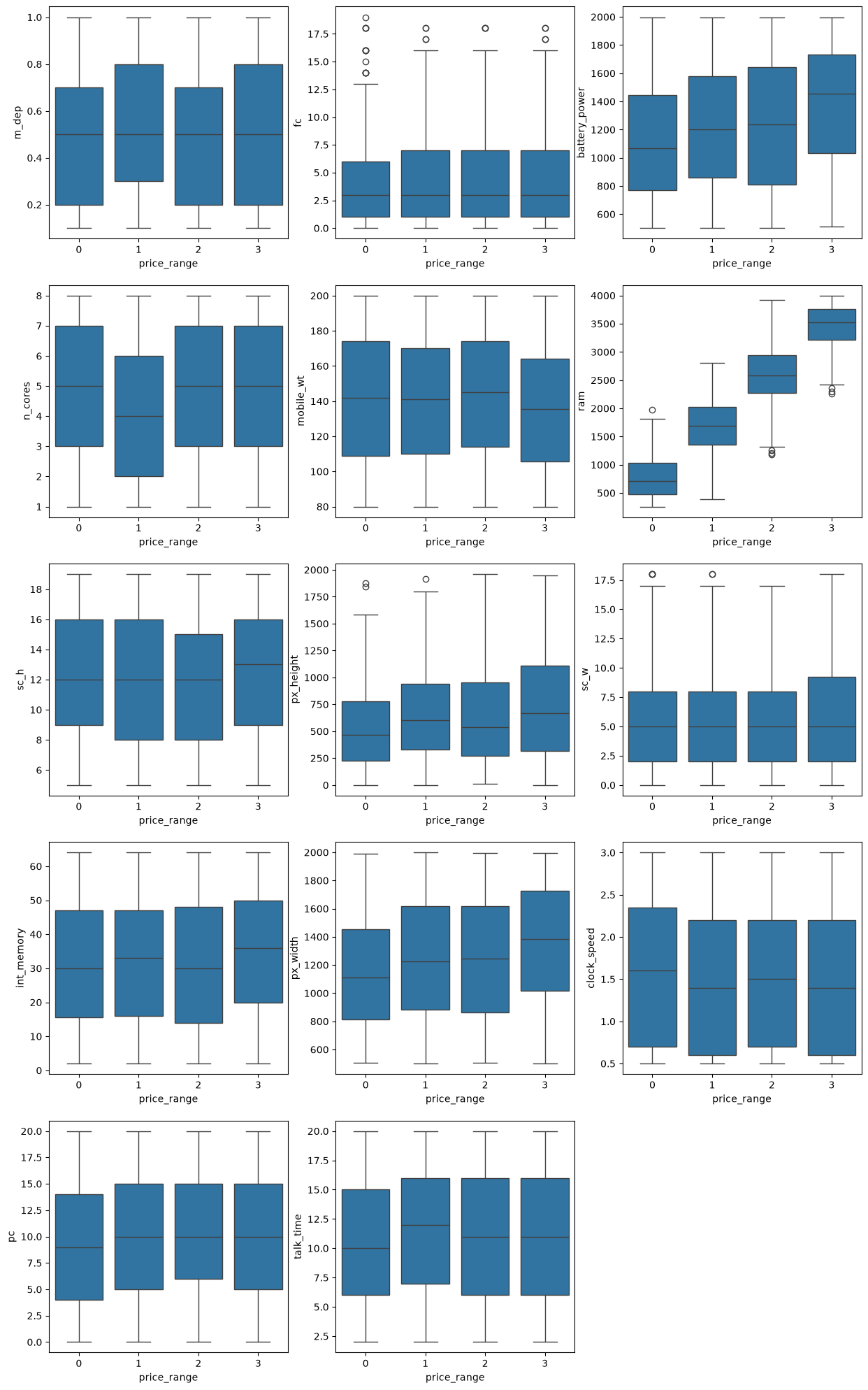

The boxplot visualization for ram demonstrates a distinct, non-overlapping ascending stair-step pattern across the target classes. The median values and interquartile ranges (IQR) for each price_range shift dramatically higher with each successive tier: - Price Range 0 (Low): Characterized by low RAM capacity (predominantly \(< 1,000 \text{ MB}\)). - Price Range 3 (Very High): Dominated exclusively by high RAM capacity (approaching \(3,000 - 4,000 \text{ MB}\)).

The absence of overlapping medians confirms that RAM alone provides near-perfect linear separability among the four price classes.

To determine which continuous numerical features hold significant predictive power over the categorical target variable (price_range), an Analysis of Variance (ANOVA) F-test is employed. Mathematically, ANOVA evaluates whether the mean of each continuous numerical features differs significantly across all ofthe classes in the target variable. The statistical hypotheses for this evaluation are formulated as follows:

Null Hypothesis (\(H_0\)): The mean of a continuous numerical features is identical across all classes in the target variable.
Alternative Hypothesis (\(H_1\)): At least one class’ mean is significantly different from the others.

A stringent significance threshold of \(\alpha = 0.05\) is applied. Categorical features that yield a \(p\text{-value} < 0.05\) allow us to rigorously reject the null hypothesis, confirming that the variance between the category means is statistically significant and not due to random chance. These verified features are selected for downstream dummy encoding and modeling, while non-significant features are discarded to keep the model parsimonious.

How Simple Comparison of Group Means Can Dictate The Relationship between Numerical and Categorical Data

If we discover that the mean of a numerical feature in price_range 0 is structurally different from price_range 1, price_range 2, and price_range 3, it demonstrates that knowing the value of that numerical feature provides immediate information about the target’s class. Mathematically, this implies that the variance between the groups is much larger than the variance within the groups.

from scipy import stats

anova_df = X_train_num_df.copy()
anova_df[target] = y_train

anova_results = []

print('----- Running ANOVA Test -----\n')

for column in num_columns:

    unique_cats = anova_df[target].unique()
    
    grouped_data = [anova_df[anova_df[target] == cat][column].values for cat in unique_cats]

    f_stat, p_val = stats.f_oneway(*grouped_data)
    
    anova_results.append({
        'Feature': column,
        'F-Statistic': f_stat,
        'P-Value': p_val
    })

# convert to DataFrame and sort by F_Statistics in descending order
anova_summary_df = pd.DataFrame(anova_results).sort_values(by='F-Statistic', ascending=False).reset_index(drop=True)

print('Results:\n')
print(anova_summary_df)

# select features with p-value < 0.05
selected_num = anova_summary_df[anova_summary_df['P-Value'] < 0.05]['Feature'].tolist()
print(f'\nSelected Numerical Features: {selected_num}\n')
print(f'Number of Selected Numerical Features: {len(selected_num)} Out of {len(num_columns)} Numerical Features.')

----- Running ANOVA Test -----

Results:

          Feature  F-Statistic       P-Value
0             ram  2760.069393  0.000000e+00
1   battery_power    23.083657  1.255203e-14
2        px_width    16.183182  2.302349e-10
3       px_height    14.065180  4.736223e-09
4      int_memory     4.981509  1.922441e-03
5       mobile_wt     3.197662  2.262644e-02
6            sc_h     2.072448  1.019529e-01
7         n_cores     1.595945  1.884610e-01
8           m_dep     1.574918  1.935476e-01
9       talk_time     1.500694  2.125445e-01
10             fc     1.061214  3.644836e-01
11    clock_speed     1.037116  3.750794e-01
12           sc_w     0.988743  3.971462e-01
13             pc     0.780857  5.046006e-01

Selected Numerical Features: ['ram', 'battery_power', 'px_width', 'px_height', 'int_memory', 'mobile_wt']

Number of Selected Numerical Features: 6 Out of 14 Numerical Features.

The One-Way ANOVA test yields an exceptionally massive F-statistic for ram alongside an empirical \(p\text{-value} \approx 0.0\) (far below the standard \(\alpha = 0.05\) threshold). This indicates that the variance between price class means for RAM is extraordinarily large compared to the variance within each class, formally establishing ram as the single most statistically significant feature in the dataset.

Numerical Features Standardization

As observed in the plots for numerical features, the numerical features exhibit vastly different scales and measurement ranges. One of the models that will be used here is K-Nearest Neighbor which is highly sensitive to these scale discrepancies because the optimization algorithm might inadvertently penalize or over-allocate weight to features with larger absolute magnitudes.

To mitigate this, StandardScaler is applied to transform all numerical features to possess a mean of 0 and a standard deviation of 1 (\(\mu = 0, \sigma = 1\)).

from sklearn.preprocessing import StandardScaler

X_test_num_df = X_test_df[num_columns]

scaler = StandardScaler()
X_train_num = X_train_num_df.values
X_test_num = X_test_num_df.values

X_train_num_scaled = scaler.fit_transform(X_train_num)
X_test_num_scaled = scaler.transform(X_test_num)

X_train_num_scaled_df = pd.DataFrame(data=X_train_num_scaled, columns=num_columns)
X_test_num_scaled_df = pd.DataFrame(data=X_test_num_scaled, columns=num_columns)

print(f'X_train_num_scaled_df shape: {X_train_num_scaled_df.shape}')
print(f'X_test_num_scaled_df shape: {X_test_num_scaled_df.shape}')

X_train_num_scaled_df shape: (1600, 14)
X_test_num_scaled_df shape: (400, 14)

X_train_num_scaled_df.head()

	m_dep	fc	battery_power	n_cores	mobile_wt	ram	sc_h	px_height	sc_w	int_memory	px_width	clock_speed	pc	talk_time
0	-0.008935	0.620111	1.548360	-1.547446	1.425710	-0.580476	-0.528061	0.275712	0.759509	0.754832	1.181997	-1.236230	0.020269	-1.445123
1	-1.403674	-0.993561	-1.379535	1.510316	-0.046246	1.336453	-0.290196	-0.258762	-1.084869	0.919763	-0.556547	0.837112	-1.476497	0.915929
2	-1.403674	-0.532512	-0.010914	-1.547446	1.340790	-0.657302	0.423400	-0.285711	1.451150	1.359577	-1.020159	-0.748385	0.685498	1.642407
3	-0.357620	-0.532512	-1.043621	0.199847	1.623858	1.288322	0.185535	-0.764042	0.528962	0.315017	0.984962	-0.504462	-0.478653	-1.081884
4	-0.357620	0.620111	0.488416	0.199847	-1.008680	-0.489767	-1.479523	0.401470	-0.162680	-1.389265	-0.336332	-1.236230	0.352883	1.642407

X_test_num_scaled_df.head()

	m_dep	fc	battery_power	n_cores	mobile_wt	ram	sc_h	px_height	sc_w	int_memory	px_width	clock_speed	pc	talk_time
0	0.339750	-0.301987	0.919657	-1.110623	1.680472	-1.323738	-1.003792	-0.972891	0.067867	-0.399682	0.831970	1.202995	-0.811268	0.007832
1	-0.008935	0.620111	-0.133477	1.510316	-0.074553	0.413624	1.612728	-0.829167	2.603886	-1.334288	-0.609863	-1.236230	1.018112	1.460787
2	-0.357620	1.081160	1.659574	1.073493	1.567245	-0.740606	-1.003792	-0.788745	-1.084869	-1.004427	-0.688677	1.690840	1.350727	-0.537026
3	-1.054989	-0.071463	-0.571527	-0.673800	0.718039	1.643754	1.374862	-0.871835	0.298414	-0.839496	0.335906	0.593189	1.517034	1.460787
4	-0.008935	0.620111	-1.420389	0.199847	-0.301008	-0.194499	0.423400	0.846117	-0.162680	1.414554	1.643291	-1.236230	-0.312346	-1.081884

# full and unscaled: X_train_df, X_test_df

# full and scaled
X_train_full_scaled_df = pd.concat([X_train_cat_df.reset_index(drop=True), X_train_num_scaled_df.reset_index(drop=True)], axis=1).sort_index(axis=1)
X_test_full_scaled_df = pd.concat([X_test_df[cat_columns].reset_index(drop=True), X_test_num_scaled_df.reset_index(drop=True)], axis=1).sort_index(axis=1)

# selected and unscaled
selected_columns = selected_num + selected_cat
X_train_selected_df = X_train_df[selected_columns].sort_index(axis=1)
X_test_selected_df = X_test_df[selected_columns].sort_index(axis=1)

# selected and scaled
X_train_selected_scaled_df = X_train_full_scaled_df[selected_columns].sort_index(axis=1)
X_test_selected_scaled_df = X_test_full_scaled_df[selected_columns].sort_index(axis=1)

print(f'X_train_full_scaled_df shape: {X_train_full_scaled_df.shape}')
print(f'X_test_full_scaled_df shape: {X_test_full_scaled_df.shape}')
print(f'X_train_selected_df shape: {X_train_selected_df.shape}')
print(f'X_test_selected_df shape: {X_test_selected_df.shape}')
print(f'X_train_selected_scaled_df shape: {X_train_selected_scaled_df.shape}')
print(f'X_test_selected_scaled_df shape: {X_test_selected_scaled_df.shape}')

X_train_full_scaled_df shape: (1600, 20)
X_test_full_scaled_df shape: (400, 20)
X_train_selected_df shape: (1600, 6)
X_test_selected_df shape: (400, 6)
X_train_selected_scaled_df shape: (1600, 6)
X_test_selected_scaled_df shape: (400, 6)

X_train_full_scaled_df.head()

	battery_power	blue	clock_speed	dual_sim	fc	four_g	int_memory	m_dep	mobile_wt	n_cores	pc	px_height	px_width	ram	sc_h	sc_w	talk_time	three_g	touch_screen	wifi
0	1.548360	0	-1.236230	1	0.620111	0	0.754832	-0.008935	1.425710	-1.547446	0.020269	0.275712	1.181997	-0.580476	-0.528061	0.759509	-1.445123	1	1	1
1	-1.379535	1	0.837112	0	-0.993561	1	0.919763	-1.403674	-0.046246	1.510316	-1.476497	-0.258762	-0.556547	1.336453	-0.290196	-1.084869	0.915929	1	1	1
2	-0.010914	0	-0.748385	1	-0.532512	1	1.359577	-1.403674	1.340790	-1.547446	0.685498	-0.285711	-1.020159	-0.657302	0.423400	1.451150	1.642407	1	0	1
3	-1.043621	0	-0.504462	0	-0.532512	0	0.315017	-0.357620	1.623858	0.199847	-0.478653	-0.764042	0.984962	1.288322	0.185535	0.528962	-1.081884	0	0	1
4	0.488416	1	-1.236230	1	0.620111	0	-1.389265	-0.357620	-1.008680	0.199847	0.352883	0.401470	-0.336332	-0.489767	-1.479523	-0.162680	1.642407	1	0	1

X_train_selected_df.head()

	battery_power	int_memory	mobile_wt	px_height	px_width	ram
968	1923	46	191	767	1759	1489
240	633	49	139	529	1009	3560
819	1236	57	188	517	809	1406
692	781	38	198	304	1674	3508
420	1456	7	105	823	1104	1587

X_train_selected_scaled_df.head()

	battery_power	int_memory	mobile_wt	px_height	px_width	ram
0	1.548360	0.754832	1.425710	0.275712	1.181997	-0.580476
1	-1.379535	0.919763	-0.046246	-0.258762	-0.556547	1.336453
2	-0.010914	1.359577	1.340790	-0.285711	-1.020159	-0.657302
3	-1.043621	0.315017	1.623858	-0.764042	0.984962	1.288322
4	0.488416	-1.389265	-1.008680	0.401470	-0.336332	-0.489767

Run The Experiment: Train and Evaluate Models Using Hyperparameter Tuning

from sklearn.neighbors import KNeighborsClassifier
from sklearn.tree import DecisionTreeClassifier
from sklearn.ensemble import RandomForestClassifier
from xgboost import XGBClassifier
from sklearn.model_selection import KFold, GridSearchCV


experiments = [
    # knn experiments
    {
        'name': 'KNN_Full_Features',
        'model': KNeighborsClassifier(),
        'use_selected_features': False,
        'needs_scaling': True,
        'params': {
            'n_neighbors': [3, 5, 7, 9, 11, 13, 15, 17, 19, 21],
        }
    },
    {
        'name': 'KNN_Feature_Selection',
        'model': KNeighborsClassifier(),
        'use_selected_features': True,
        'needs_scaling': True,
        'params': {
            'n_neighbors': [3, 5, 7, 9, 11, 13, 15, 17, 19, 21],
        }
    },
    
    # decision tree Experiments
    {
        'name': 'DecisionTree_Full_Features',
        'model': DecisionTreeClassifier(random_state=42),
        'use_selected_features': False,
        'needs_scaling': False,
        'params': {
            'criterion': ['gini', 'entropy'],
            'max_depth': [None, 3, 5, 7, 10]
        }
    },
    {
        'name': 'DecisionTree_Feature_Selection',
        'model': DecisionTreeClassifier(random_state=42),
        'use_selected_features': True,
        'needs_scaling': False,
        'params': {
            'criterion': ['gini', 'entropy'],
            'max_depth': [None, 3, 5, 7, 10]
        }
    },

    # random forest experiments
    {
        'name': 'RandomForest_Full_Features',
        'model': RandomForestClassifier(random_state=42),
        'use_selected_features': False,
        'needs_scaling': False,
        'params': {
            'criterion': ['gini', 'entropy'],
            'max_depth': [None, 3, 5, 7, 10],
            'n_estimators': [100, 200, 300, 400, 500]
        }
    },
    {
        'name': 'RandomForest_Feature_Selection',
        'model': RandomForestClassifier(random_state=42),
        'use_selected_features': True,
        'needs_scaling': False,
        'params': {
            'criterion': ['gini', 'entropy'],
            'max_depth': [None, 3, 5, 7, 10],
            'n_estimators': [100, 200, 300, 400, 500]
        }
    },

    # xgboost experiments
    {
        'name': 'XGBoost_Full_Features',
        'model': XGBClassifier(objective='multi:softprob', num_class=4, random_state=42),
        'use_selected_features': False,
        'needs_scaling': False,
        'params': {
            'n_estimators': [50, 100, 200],
            'learning_rate': [0.01, 0.05, 0.1, 0.2],
            'max_depth': [3, 5, 7]
        }
    },
    {
        'name': 'XGBoost_Feature_Selection',
        'model': XGBClassifier(objective='multi:softprob', num_class=4, random_state=42),
        'use_selected_features': True,
        'needs_scaling': False,
        'params': {
            'n_estimators': [50, 100, 200],
            'learning_rate': [0.01, 0.05, 0.1, 0.2],
            'max_depth': [3, 5, 7]
        }
    }
]

results_list = []

for exp in experiments:
    print(f'Running Experiment: {exp['name']}')

    kf = KFold(n_splits=5, shuffle=True, random_state=42)

    grid_cv = GridSearchCV(
        estimator=exp['model'],
        param_grid=exp['params'],
        cv=kf,
        scoring='accuracy',
        n_jobs=-1
    )

    if exp['use_selected_features']:
        if exp['needs_scaling']:
            X_train =  X_train_selected_scaled_df.values
            X_test = X_test_selected_scaled_df.values
        else:
            X_train =  X_train_selected_df.values
            X_test = X_test_selected_df.values
    else:
        if exp['needs_scaling']:
            X_train = X_train_full_scaled_df.values
            X_test = X_test_full_scaled_df.values
        else:
            X_train = X_train_df.values
            X_test = X_test_df.values
            
    grid_cv.fit(X_train, y_train)
    best_model = grid_cv.best_estimator_
    test_accuracy = best_model.score(X_test, y_test)
    
    results_list.append({
        'Experiment': exp['name'],
        'Best Parameters': grid_cv.best_params_,
        'Best CV Score': grid_cv.best_score_,
        'Test Accuracy': test_accuracy
    })

# Convert summary into DataFrame for notebook presentation
results_df = pd.DataFrame(results_list)
results_df

Running Experiment: KNN_Full_Features
Running Experiment: KNN_Feature_Selection
Running Experiment: DecisionTree_Full_Features
Running Experiment: DecisionTree_Feature_Selection
Running Experiment: RandomForest_Full_Features
Running Experiment: RandomForest_Feature_Selection
Running Experiment: XGBoost_Full_Features
Running Experiment: XGBoost_Feature_Selection

	Experiment	Best Parameters	Best CV Score	Test Accuracy
0	KNN_Full_Features	{'n_neighbors': 21}	0.646875	0.6850
1	KNN_Feature_Selection	{'n_neighbors': 19}	0.803750	0.8175
2	DecisionTree_Full_Features	{'criterion': 'entropy', 'max_depth': None}	0.855625	0.8500
3	DecisionTree_Feature_Selection	{'criterion': 'entropy', 'max_depth': None}	0.868750	0.8475
4	RandomForest_Full_Features	{'criterion': 'entropy', 'max_depth': None, 'n...	0.889375	0.9000
5	RandomForest_Feature_Selection	{'criterion': 'gini', 'max_depth': None, 'n_es...	0.913125	0.9275
6	XGBoost_Full_Features	{'learning_rate': 0.2, 'max_depth': 3, 'n_esti...	0.915000	0.9175
7	XGBoost_Feature_Selection	{'learning_rate': 0.2, 'max_depth': 3, 'n_esti...	0.921875	0.9125

The empirical results from the 8 experimental configurations provide critical insights into algorithmic behavior and the impact of statistical feature selection on high-dimensional tabular data.

Key Findings & Insights:

The Dramatic Impact of Feature Selection on KNN:
- KNN_Full_Features: Achieved the lowest performance (\(\text{CV: } 64.69\%, \text{ Test: } 68.50\%\)). The presence of 20 baseline features severely degraded distance-based metrics due to the curse of dimensionality and noisy categorical attributes.
- KNN_Feature_Selection: Performance jumped significantly (\(\text{CV: } 80.38\%, \text{ Test: } 81.75\%\)), yielding a +13.25% improvement in Test Accuracy. Pruning non-informative variables directly refined the Euclidean distance space.
Resilience of Tree-Based Models:
- Single Decision Trees (DecisionTree) exhibited stable performance (\(\sim 84.75\% - 85.00\%\) Test Accuracy) across both feature sets, proving their native ability to prioritize splits based on Information Gain/Entropy (criterion='entropy').
Dominance of Ensemble Methods (Random Forest & XGBoost):
- Ensemble frameworks consistently outperformed single estimators, crossing the \(90\%\) accuracy threshold.
- Random Forest with Feature Selection achieved the highest overall test accuracy of \(92.75\%\) (\(\text{CV: } 91.31\%\)), demonstrating that eliminating low-variance noise features allows bagging ensembles to build higher-quality decision boundaries.
- XGBoost maintained exceptionally tight convergence between CV score and Test Accuracy (\(\sim 91.25\% - 92.18\%\)), highlighting the robustness of gradient boosting against variance.

When evaluating the top-performing models, a classic trade-off between Peak Test Accuracy and Generalization Stability emerges:

XGBoost_Full_Features demonstrates superior variance control, achieving a remarkably narrow generalization gap of \(0.25\%\) (\(\text{CV: } 91.50\% \text{ vs Test: } 91.75\%\)). This confirms that gradient boosting seamlessly manages baseline noise across data splits.
RandomForest_Feature_Selection, however, delivers the highest absolute classification accuracy on unseen data (\(92.75\%\)) while maintaining a healthy, non-overfitting gap of \(1.44\%\).

Conclusion: RandomForest_Feature_Selection is recommended as the primary candidate due to its superior predictive capability (\(+1.00\%\) accuracy over XGBoost) and lower feature complexity (adhering to Occam’s Razor by discarding non-informative features). Nonetheless, XGBoost_Full_Features stands as a highly robust alternative for environments prioritizing strict cross-split stability.

best_model_id = 5
best_model_name = results_df['Experiment'].iloc[best_model_id]
best_params = results_df['Best Parameters'].iloc[best_model_id]

print(f'Best Model: {best_model_name}')
print(f'Best Parameters: {best_params}')

model = experiments[best_model_id]['model'].set_params(**best_params)

exp = experiments[best_model_id]
if exp['use_selected_features']:
    if exp['needs_scaling']:
        X_train =  X_train_selected_scaled_df.values
        X_test = X_test_selected_scaled_df.values
    else:
        X_train =  X_train_selected_df.values
        X_test = X_test_selected_df.values
else:
    if exp['needs_scaling']:
        X_train = X_train_full_scaled_df.values
        X_test = X_test_full_scaled_df.values
    else:
        X_train = X_train_df.values
        X_test = X_test_df.values

model.fit(X_train, y_train)

Best Model: RandomForest_Feature_Selection
Best Parameters: {'criterion': 'gini', 'max_depth': None, 'n_estimators': 200}

RandomForestClassifier(n_estimators=200, random_state=42)

In a Jupyter environment, please rerun this cell to show the HTML representation or trust the notebook.
On GitHub, the HTML representation is unable to render, please try loading this page with nbviewer.org.

RandomForestClassifier

?Documentation for RandomForestClassifieriFitted

Parameters

	n_estimators n_estimators: int, default=100 The number of trees in the forest. .. versionchanged:: 0.22 The default value of ``n_estimators`` changed from 10 to 100 in 0.22.	200
	random_state random_state: int, RandomState instance or None, default=None Controls both the randomness of the bootstrapping of the samples used when building trees (if ``bootstrap=True``) and the sampling of the features to consider when looking for the best split at each node (if ``max_features < n_features``). See :term:`Glossary <random_state>` for details.	42
	criterion criterion: {"gini", "entropy", "log_loss"}, default="gini" The function to measure the quality of a split. Supported criteria are "gini" for the Gini impurity and "log_loss" and "entropy" both for the Shannon information gain, see :ref:`tree_mathematical_formulation`. Note: This parameter is tree-specific.	'gini'
	max_depth max_depth: int, default=None The maximum depth of the tree. If None, then nodes are expanded until all leaves are pure or until all leaves contain less than min_samples_split samples.	None
	min_samples_split min_samples_split: int or float, default=2 The minimum number of samples required to split an internal node: - If int, then consider `min_samples_split` as the minimum number. - If float, then `min_samples_split` is a fraction and `ceil(min_samples_split * n_samples)` are the minimum number of samples for each split. .. versionchanged:: 0.18 Added float values for fractions.	2
	min_samples_leaf min_samples_leaf: int or float, default=1 The minimum number of samples required to be at a leaf node. A split point at any depth will only be considered if it leaves at least ``min_samples_leaf`` training samples in each of the left and right branches. This may have the effect of smoothing the model, especially in regression. - If int, then consider `min_samples_leaf` as the minimum number. - If float, then `min_samples_leaf` is a fraction and `ceil(min_samples_leaf * n_samples)` are the minimum number of samples for each node. .. versionchanged:: 0.18 Added float values for fractions.	1
	min_weight_fraction_leaf min_weight_fraction_leaf: float, default=0.0 The minimum weighted fraction of the sum total of weights (of all the input samples) required to be at a leaf node. Samples have equal weight when sample_weight is not provided.	0.0
	max_features max_features: {"sqrt", "log2", None}, int or float, default="sqrt" The number of features to consider when looking for the best split: - If int, then consider `max_features` features at each split. - If float, then `max_features` is a fraction and `max(1, int(max_features * n_features_in_))` features are considered at each split. - If "sqrt", then `max_features=sqrt(n_features)`. - If "log2", then `max_features=log2(n_features)`. - If None, then `max_features=n_features`. .. versionchanged:: 1.1 The default of `max_features` changed from `"auto"` to `"sqrt"`. Note: the search for a split does not stop until at least one valid partition of the node samples is found, even if it requires to effectively inspect more than ``max_features`` features.	'sqrt'
	max_leaf_nodes max_leaf_nodes: int, default=None Grow trees with ``max_leaf_nodes`` in best-first fashion. Best nodes are defined as relative reduction in impurity. If None then unlimited number of leaf nodes.	None
	min_impurity_decrease min_impurity_decrease: float, default=0.0 A node will be split if this split induces a decrease of the impurity greater than or equal to this value. The weighted impurity decrease equation is the following:: N_t / N * (impurity - N_t_R / N_t * right_impurity - N_t_L / N_t * left_impurity) where ``N`` is the total number of samples, ``N_t`` is the number of samples at the current node, ``N_t_L`` is the number of samples in the left child, and ``N_t_R`` is the number of samples in the right child. ``N``, ``N_t``, ``N_t_R`` and ``N_t_L`` all refer to the weighted sum, if ``sample_weight`` is passed. .. versionadded:: 0.19	0.0
	bootstrap bootstrap: bool, default=True Whether bootstrap samples are used when building trees. If False, the whole dataset is used to build each tree.	True
	oob_score oob_score: bool or callable, default=False Whether to use out-of-bag samples to estimate the generalization score. By default, :func:`~sklearn.metrics.accuracy_score` is used. Provide a callable with signature `metric(y_true, y_pred)` to use a custom metric. Only available if `bootstrap=True`. For an illustration of out-of-bag (OOB) error estimation, see the example :ref:`sphx_glr_auto_examples_ensemble_plot_ensemble_oob.py`.	False
	n_jobs n_jobs: int, default=None The number of jobs to run in parallel. :meth:`fit`, :meth:`predict`, :meth:`decision_path` and :meth:`apply` are all parallelized over the trees. ``None`` means 1 unless in a :obj:`joblib.parallel_backend` context. ``-1`` means using all processors. See :term:`Glossary <n_jobs>` for more details.	None
	verbose verbose: int, default=0 Controls the verbosity when fitting and predicting.	0
	warm_start warm_start: bool, default=False When set to ``True``, reuse the solution of the previous call to fit and add more estimators to the ensemble, otherwise, just fit a whole new forest. See :term:`Glossary <warm_start>` and :ref:`tree_ensemble_warm_start` for details.	False
	class_weight class_weight: {"balanced", "balanced_subsample"}, dict or list of dicts, default=None Weights associated with classes in the form ``{class_label: weight}``. If not given, all classes are supposed to have weight one. For multi-output problems, a list of dicts can be provided in the same order as the columns of y. Note that for multioutput (including multilabel) weights should be defined for each class of every column in its own dict. For example, for four-class multilabel classification weights should be [{0: 1, 1: 1}, {0: 1, 1: 5}, {0: 1, 1: 1}, {0: 1, 1: 1}] instead of [{1:1}, {2:5}, {3:1}, {4:1}]. The "balanced" mode uses the values of y to automatically adjust weights inversely proportional to class frequencies in the input data as ``n_samples / (n_classes * np.bincount(y))`` The "balanced_subsample" mode is the same as "balanced" except that weights are computed based on the bootstrap sample for every tree grown. For multi-output, the weights of each column of y will be multiplied. Note that these weights will be multiplied with sample_weight (passed through the fit method) if sample_weight is specified.	None
	ccp_alpha ccp_alpha: non-negative float, default=0.0 Complexity parameter used for Minimal Cost-Complexity Pruning. The subtree with the largest cost complexity that is smaller than ``ccp_alpha`` will be chosen. By default, no pruning is performed. See :ref:`minimal_cost_complexity_pruning` for details. See :ref:`sphx_glr_auto_examples_tree_plot_cost_complexity_pruning.py` for an example of such pruning. .. versionadded:: 0.22	0.0
	max_samples max_samples: int or float, default=None If bootstrap is True, the number of samples to draw from X to train each base estimator. - If None (default), then draw `X.shape[0]` samples irrespective of `sample_weight`. - If int, then draw `max_samples` samples. - If float, then draw `max_samples * X.shape[0]` unweighted samples or `max_samples * sample_weight.sum()` weighted samples. .. versionadded:: 0.22 .. versionchanged:: 1.9 Float `max_samples` is relative to `sample_weight.sum()` instead of `X.shape[0]` for weighted samples.	None
	monotonic_cst monotonic_cst: array-like of int of shape (n_features), default=None Indicates the monotonicity constraint to enforce on each feature. - 1: monotonic increase - 0: no constraint - -1: monotonic decrease If monotonic_cst is None, no constraints are applied. Monotonicity constraints are not supported for: - multiclass classifications (i.e. when `n_classes > 2`), - multioutput classifications (i.e. when `n_outputs_ > 1`). The constraints hold over the probability of the positive class. Read more in the :ref:`User Guide <monotonic_cst_gbdt>`. .. versionadded:: 1.4	None

Fitted attributes

Name	Type	Value
classes_ classes_: ndarray of shape (n_classes,) or a list of such arrays The classes labels (single output problem), or a list of arrays of class labels (multi-output problem).	ndarray[int64](4,)	[0,1,2,3]
estimator_ estimator_: :class:`~sklearn.tree.DecisionTreeClassifier` The child estimator template used to create the collection of fitted sub-estimators. .. versionadded:: 1.2 `base_estimator_` was renamed to `estimator_`.	DecisionTreeClassifier	DecisionTreeClassifier()
estimators_ estimators_: list of DecisionTreeClassifier The collection of fitted sub-estimators.	list	[DecisionTreeC...te=1608637542), DecisionTreeC...te=1273642419), DecisionTreeC...te=1935803228), DecisionTreeC...ate=787846414), ...]
estimators_samples_ estimators_samples_: list of arrays The subset of drawn samples (i.e., the in-bag samples) for each base estimator. Each subset is defined by an array of the indices selected. .. versionadded:: 1.4	list	[array([ 475, ..., dtype=int32), array([ 686, ..., dtype=int32), array([1366, ..., dtype=int32), array([ 800, ..., dtype=int32), ...]
feature_importances_ feature_importances_: ndarray of shape (n_features,) The impurity-based feature importances. The higher, the more important the feature. The importance of a feature is computed as the (normalized) total reduction of the criterion brought by that feature. It is also known as the Gini importance. Warning: impurity-based feature importances can be misleading for high cardinality features (many unique values). See :func:`sklearn.inspection.permutation_importance` as an alternative.	ndarray[float64](6,)	[0.11,0.05,0.05,0.08,0.08,0.63]
n_classes_ n_classes_: int or list The number of classes (single output problem), or a list containing the number of classes for each output (multi-output problem).	int	4
n_features_in_ n_features_in_: int Number of features seen during :term:`fit`. .. versionadded:: 0.24	int	6
n_outputs_ n_outputs_: int The number of outputs when ``fit`` is performed.	int	1

y_pred = model.predict(X_test)
y_pred

array([0, 2, 1, 3, 1, 1, 2, 0, 3, 1, 0, 1, 2, 3, 2, 2, 3, 3, 1, 0, 0, 1,
       1, 2, 0, 1, 3, 2, 2, 0, 0, 0, 3, 0, 1, 1, 2, 0, 3, 0, 2, 3, 2, 0,
       3, 2, 1, 1, 3, 1, 3, 1, 0, 0, 1, 1, 1, 3, 0, 0, 1, 3, 3, 1, 0, 0,
       3, 3, 1, 2, 2, 2, 0, 1, 2, 0, 0, 3, 2, 2, 3, 2, 1, 0, 1, 3, 1, 3,
       3, 0, 3, 3, 2, 1, 3, 2, 2, 3, 1, 1, 0, 0, 1, 0, 0, 3, 2, 0, 1, 1,
       0, 0, 3, 1, 2, 2, 3, 3, 0, 2, 1, 3, 2, 1, 3, 3, 0, 3, 0, 2, 3, 0,
       2, 2, 0, 3, 1, 0, 0, 2, 3, 1, 2, 2, 0, 0, 0, 1, 1, 2, 3, 1, 1, 0,
       2, 2, 0, 1, 0, 1, 2, 3, 3, 2, 1, 0, 1, 2, 2, 3, 3, 1, 1, 0, 3, 1,
       1, 2, 1, 0, 0, 0, 0, 0, 3, 2, 0, 3, 0, 0, 0, 0, 1, 3, 3, 1, 0, 1,
       1, 1, 1, 2, 2, 2, 3, 3, 1, 2, 0, 0, 0, 2, 1, 1, 3, 1, 0, 2, 1, 1,
       3, 2, 3, 0, 0, 2, 1, 2, 0, 1, 2, 0, 2, 3, 2, 1, 1, 3, 3, 0, 1, 3,
       3, 3, 0, 3, 1, 2, 3, 3, 2, 1, 1, 3, 3, 1, 3, 3, 3, 3, 3, 0, 1, 2,
       2, 1, 2, 0, 2, 3, 2, 2, 2, 1, 0, 2, 0, 3, 3, 1, 3, 1, 0, 3, 1, 2,
       0, 0, 3, 0, 1, 2, 3, 3, 3, 1, 1, 0, 1, 3, 3, 0, 1, 2, 2, 0, 3, 3,
       2, 3, 2, 3, 2, 0, 2, 1, 1, 1, 0, 0, 0, 3, 2, 3, 1, 0, 1, 0, 1, 3,
       3, 0, 3, 3, 2, 1, 3, 0, 0, 3, 1, 3, 2, 0, 1, 1, 1, 1, 1, 3, 1, 0,
       0, 3, 3, 0, 3, 0, 0, 2, 0, 1, 2, 2, 2, 3, 0, 3, 2, 2, 3, 3, 3, 2,
       1, 2, 0, 3, 1, 3, 3, 0, 2, 3, 2, 3, 3, 3, 0, 0, 2, 3, 0, 0, 2, 3,
       2, 1, 1, 2])

from sklearn.metrics import classification_report, confusion_matrix, ConfusionMatrixDisplay

print("--- Classification Report ---")
report = classification_report(y_test, y_pred)
print('Classification Report:\n')
print(report)

print("--- Confusion Matrix ---")
cm = confusion_matrix(y_test, y_pred)
disp = ConfusionMatrixDisplay(confusion_matrix=cm)
disp.plot()

--- Classification Report ---
Classification Report:

              precision    recall  f1-score   support

           0       0.99      0.95      0.97       105
           1       0.89      0.98      0.93        91
           2       0.89      0.86      0.87        92
           3       0.94      0.92      0.93       112

    accuracy                           0.93       400
   macro avg       0.93      0.93      0.93       400
weighted avg       0.93      0.93      0.93       400

--- Confusion Matrix ---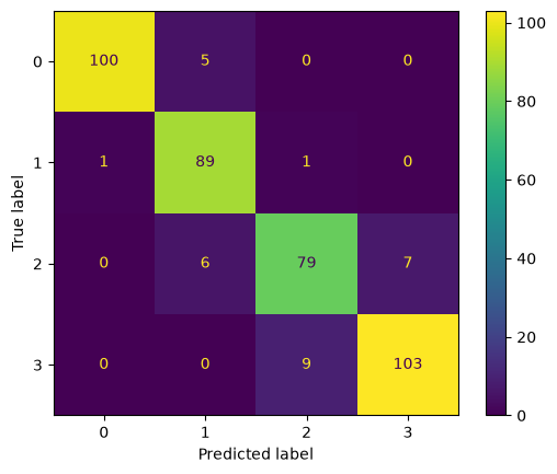

Save Best Model

import joblib

best_model_name = best_model_name.replace(' ', '_').lower()
joblib.dump(model, f'model/mobiles_{best_model_name}.pkl')

['model/mobiles_randomforest_feature_selection.pkl']

Also Save The Selected Features

with open('model/mobiles_selected_features.txt', mode='w', encoding='utf-8') as f:
    for feature in selected_columns:
        f.write(f'{feature}\n')

Use The Model to Predict Mobiles Price Range for The New Data

df_new = pd.read_csv('data/mobiles_new.csv')
df_new

	id	battery_power	blue	clock_speed	dual_sim	fc	four_g	int_memory	m_dep	mobile_wt	...	pc	px_height	px_width	ram	sc_h	sc_w	talk_time	three_g	touch_screen	wifi
0	1	1043	1	1.8	1	14	0	5	0.1	193	...	16	226	1412	3476	12	7	2	0	1	0
1	2	841	1	0.5	1	4	1	61	0.8	191	...	12	746	857	3895	6	0	7	1	0	0
2	3	1807	1	2.8	0	1	0	27	0.9	186	...	4	1270	1366	2396	17	10	10	0	1	1
3	4	1546	0	0.5	1	18	1	25	0.5	96	...	20	295	1752	3893	10	0	7	1	1	0
4	5	1434	0	1.4	0	11	1	49	0.5	108	...	18	749	810	1773	15	8	7	1	0	1
...	...	...	...	...	...	...	...	...	...	...	...	...	...	...	...	...	...	...	...	...	...
995	996	1700	1	1.9	0	0	1	54	0.5	170	...	17	644	913	2121	14	8	15	1	1	0
996	997	609	0	1.8	1	0	0	13	0.9	186	...	2	1152	1632	1933	8	1	19	0	1	1
997	998	1185	0	1.4	0	1	1	8	0.5	80	...	12	477	825	1223	5	0	14	1	0	0
998	999	1533	1	0.5	1	0	0	50	0.4	171	...	12	38	832	2509	15	11	6	0	1	0
999	1000	1270	1	0.5	0	4	1	35	0.1	140	...	19	457	608	2828	9	2	3	1	0	1

1000 rows × 21 columns

df_new.info()

<class 'pandas.DataFrame'>
RangeIndex: 1000 entries, 0 to 999
Data columns (total 21 columns):
 #   Column         Non-Null Count  Dtype  
---  ------         --------------  -----  
 0   id             1000 non-null   int64  
 1   battery_power  1000 non-null   int64  
 2   blue           1000 non-null   int64  
 3   clock_speed    1000 non-null   float64
 4   dual_sim       1000 non-null   int64  
 5   fc             1000 non-null   int64  
 6   four_g         1000 non-null   int64  
 7   int_memory     1000 non-null   int64  
 8   m_dep          1000 non-null   float64
 9   mobile_wt      1000 non-null   int64  
 10  n_cores        1000 non-null   int64  
 11  pc             1000 non-null   int64  
 12  px_height      1000 non-null   int64  
 13  px_width       1000 non-null   int64  
 14  ram            1000 non-null   int64  
 15  sc_h           1000 non-null   int64  
 16  sc_w           1000 non-null   int64  
 17  talk_time      1000 non-null   int64  
 18  three_g        1000 non-null   int64  
 19  touch_screen   1000 non-null   int64  
 20  wifi           1000 non-null   int64  
dtypes: float64(2), int64(19)
memory usage: 164.2 KB

# drop column id

df_new = df_new.drop(columns=['id'])

# load selected features from the saved txt file
selected_features = []
with open('model/mobiles_selected_features.txt', mode='r', encoding='utf-8') as f:
    for line in f:
        selected_features.append(line.strip())

# filter only selected features and sort the columns in the same order as the training data
df_new = df_new[selected_features].sort_index(axis=1)
df_new

	battery_power	int_memory	mobile_wt	px_height	px_width	ram
0	1043	5	193	226	1412	3476
1	841	61	191	746	857	3895
2	1807	27	186	1270	1366	2396
3	1546	25	96	295	1752	3893
4	1434	49	108	749	810	1773
...	...	...	...	...	...	...
995	1700	54	170	644	913	2121
996	609	13	186	1152	1632	1933
997	1185	8	80	477	825	1223
998	1533	50	171	38	832	2509
999	1270	35	140	457	608	2828

1000 rows × 6 columns

X_new = df_new.values

# load saved model
model = joblib.load('model/mobiles_randomforest_feature_selection.pkl')

# predict the price range for new data
y_new_predict = model.predict(X_new)
y_new_predict

array([3, 3, 2, 3, 1, 3, 3, 1, 3, 0, 3, 3, 0, 0, 2, 0, 2, 1, 3, 2, 1, 3,
       1, 1, 3, 0, 2, 0, 2, 0, 2, 0, 3, 0, 0, 1, 3, 1, 2, 1, 1, 2, 0, 0,
       0, 1, 0, 3, 1, 2, 1, 0, 3, 0, 3, 1, 3, 1, 1, 3, 3, 2, 0, 2, 1, 1,
       1, 3, 1, 2, 1, 2, 2, 3, 3, 0, 2, 0, 2, 3, 0, 3, 3, 0, 3, 0, 3, 1,
       3, 0, 1, 2, 2, 0, 2, 1, 0, 2, 1, 2, 1, 0, 0, 3, 1, 2, 0, 1, 2, 3,
       3, 2, 1, 3, 3, 3, 3, 2, 3, 0, 0, 3, 2, 1, 2, 0, 3, 2, 3, 1, 0, 2,
       1, 1, 3, 1, 1, 0, 3, 2, 1, 3, 1, 2, 2, 3, 3, 2, 2, 3, 2, 3, 0, 0,
       3, 2, 3, 3, 3, 3, 2, 2, 3, 3, 3, 3, 1, 0, 3, 0, 0, 0, 1, 1, 0, 1,
       0, 0, 1, 2, 1, 0, 0, 1, 1, 2, 2, 1, 0, 0, 0, 1, 0, 3, 2, 0, 2, 2,
       2, 3, 1, 2, 3, 2, 3, 2, 2, 1, 0, 0, 1, 2, 0, 2, 3, 3, 0, 2, 0, 3,
       2, 3, 3, 1, 0, 1, 0, 3, 0, 1, 0, 2, 2, 1, 2, 0, 3, 0, 3, 1, 2, 0,
       0, 2, 1, 3, 3, 3, 1, 1, 3, 0, 0, 2, 3, 3, 1, 3, 1, 1, 3, 2, 1, 2,
       3, 3, 3, 1, 0, 1, 2, 3, 2, 1, 3, 2, 0, 3, 0, 1, 2, 0, 0, 3, 2, 3,
       3, 2, 1, 3, 3, 2, 3, 2, 2, 1, 2, 0, 2, 3, 1, 0, 0, 3, 0, 3, 0, 1,
       2, 0, 2, 3, 1, 3, 2, 2, 1, 2, 0, 0, 0, 1, 3, 2, 0, 0, 0, 3, 2, 0,
       3, 3, 1, 2, 3, 2, 3, 1, 3, 3, 2, 2, 2, 3, 3, 0, 3, 0, 3, 1, 3, 1,
       3, 3, 0, 1, 1, 3, 1, 3, 2, 3, 0, 0, 0, 0, 2, 0, 0, 2, 2, 1, 2, 3,
       2, 0, 1, 0, 0, 3, 2, 0, 3, 1, 2, 2, 1, 2, 3, 1, 1, 2, 2, 1, 2, 0,
       1, 1, 0, 3, 2, 1, 0, 1, 0, 0, 1, 1, 0, 0, 0, 2, 2, 3, 2, 3, 0, 3,
       0, 3, 0, 1, 1, 1, 1, 0, 3, 2, 3, 3, 1, 3, 1, 3, 1, 3, 2, 0, 2, 2,
       1, 1, 0, 0, 0, 1, 2, 1, 0, 3, 2, 0, 2, 3, 0, 0, 3, 1, 1, 0, 3, 3,
       3, 0, 3, 0, 2, 3, 3, 3, 0, 2, 0, 2, 3, 0, 1, 1, 0, 0, 1, 1, 1, 3,
       3, 3, 2, 3, 1, 1, 2, 2, 3, 3, 2, 0, 2, 2, 2, 2, 1, 0, 2, 2, 0, 0,
       0, 3, 1, 1, 2, 2, 2, 0, 3, 0, 2, 2, 0, 3, 0, 2, 3, 0, 1, 1, 3, 3,
       1, 1, 2, 3, 2, 0, 2, 1, 2, 0, 3, 3, 1, 2, 2, 2, 3, 0, 1, 2, 3, 1,
       3, 2, 3, 1, 1, 1, 0, 3, 1, 0, 3, 2, 3, 2, 0, 3, 3, 3, 2, 3, 3, 1,
       2, 1, 2, 3, 3, 1, 0, 1, 1, 2, 2, 2, 0, 0, 2, 2, 3, 2, 0, 2, 1, 3,
       3, 0, 1, 3, 0, 2, 1, 1, 0, 0, 2, 1, 0, 1, 1, 2, 2, 0, 2, 2, 1, 0,
       3, 0, 0, 3, 2, 0, 0, 0, 0, 0, 3, 0, 3, 1, 3, 2, 1, 3, 2, 0, 1, 1,
       3, 2, 2, 2, 0, 3, 0, 2, 0, 2, 0, 1, 1, 1, 1, 2, 1, 3, 1, 3, 2, 2,
       1, 3, 2, 0, 1, 2, 0, 3, 3, 0, 2, 1, 1, 2, 0, 3, 2, 0, 3, 2, 3, 0,
       0, 3, 0, 2, 2, 3, 2, 2, 2, 2, 1, 2, 3, 0, 1, 1, 1, 2, 1, 0, 0, 1,
       0, 0, 3, 0, 1, 1, 0, 1, 1, 1, 3, 0, 3, 2, 3, 0, 0, 1, 2, 2, 1, 0,
       1, 2, 0, 1, 1, 0, 0, 3, 3, 0, 3, 1, 2, 3, 0, 1, 0, 2, 2, 0, 3, 1,
       0, 3, 0, 1, 0, 3, 3, 3, 2, 3, 0, 3, 2, 0, 1, 0, 3, 3, 2, 0, 2, 1,
       3, 1, 0, 3, 2, 0, 3, 1, 2, 1, 1, 1, 3, 1, 1, 1, 2, 0, 0, 2, 2, 0,
       2, 0, 0, 0, 0, 3, 3, 3, 3, 0, 1, 2, 2, 1, 0, 0, 2, 1, 0, 2, 0, 2,
       2, 2, 1, 2, 0, 2, 1, 3, 0, 0, 3, 1, 3, 0, 0, 2, 3, 3, 1, 2, 2, 1,
       0, 0, 2, 3, 0, 3, 0, 0, 0, 2, 2, 1, 3, 0, 3, 2, 1, 2, 3, 3, 0, 1,
       1, 2, 1, 2, 2, 0, 1, 3, 1, 1, 3, 1, 2, 3, 1, 1, 1, 1, 3, 3, 0, 2,
       3, 0, 2, 3, 2, 2, 2, 3, 2, 0, 1, 2, 0, 2, 1, 1, 2, 2, 2, 1, 2, 1,
       1, 1, 3, 1, 0, 1, 2, 3, 1, 0, 0, 3, 2, 2, 3, 0, 3, 3, 2, 1, 3, 0,
       1, 3, 1, 2, 1, 2, 3, 2, 0, 3, 0, 2, 3, 0, 3, 2, 2, 3, 1, 0, 2, 3,
       1, 0, 2, 1, 2, 1, 3, 0, 2, 2, 0, 2, 3, 2, 3, 0, 2, 1, 1, 2, 2, 3,
       3, 0, 2, 1, 2, 1, 3, 0, 1, 3, 0, 1, 0, 0, 3, 2, 2, 0, 0, 0, 0, 3,
       2, 3, 3, 0, 0, 2, 1, 0, 2, 2])

df_new['predicted_price_range'] = y_new_predict
df_new

	battery_power	int_memory	mobile_wt	px_height	px_width	ram	predicted_price_range
0	1043	5	193	226	1412	3476	3
1	841	61	191	746	857	3895	3
2	1807	27	186	1270	1366	2396	2
3	1546	25	96	295	1752	3893	3
4	1434	49	108	749	810	1773	1
...	...	...	...	...	...	...	...
995	1700	54	170	644	913	2121	2
996	609	13	186	1152	1632	1933	1
997	1185	8	80	477	825	1223	0
998	1533	50	171	38	832	2509	2
999	1270	35	140	457	608	2828	2

1000 rows × 7 columns

# save results to a new csv file
df_new.to_csv('data/mobiles_new_predicted.csv', index=False)